基于WIN10的64位系统演示
一、写在前面
(1)预训练模型和迁移学习
预训练模型就像是一个精心制作的省力工具,它是在大量的数据上进行训练,然后将学习到的模型参数保存下来。然后,我们可以直接使用这些参数,而不需要从头开始训练模型。这样可以节省大量的时间和计算资源。
那么,迁移学习呢?迁移学习就像是我们生活中的二手市场。在二手市场中,你可以买到别人已经不再使用,但是还处于良好状态的物品。这些物品可以直接用于你的需要,或者经过一些小修改后使用。同样,迁移学习就是将在一个任务上训练好的模型应用到另一个任务上。具体来说,我们可以将预训练模型的参数作为新任务的初始参数,然后在新的数据上继续训练模型。这样,我们不仅可以利用预训练模型学习到的知识,还可以根据新任务的需求,微调模型的参数。
(2)VGG19
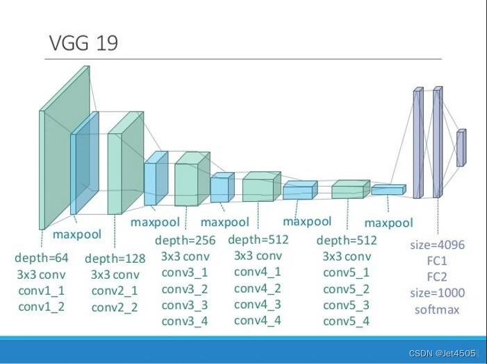
VGG19 是一个深度卷积神经网络,由牛津大学的 Visual Geometry Group 开发并命名。这个名字中的 "19" 代表着它的网络深度——总共有 19 层,这包括卷积层和全连接层。
这个模型在一系列的图像处理任务中表现得非常出色,包括图像分类、物体检测和语义分割等。VGG19 的一个显著特点是其结构的简洁和统一。它主要由一系列的卷积层和池化层堆叠而成,其中每个卷积层都使用相同大小的滤波器,并且每两个卷积层之间都插入了一个池化层。这样的设计使得 VGG19 既可以有效地提取图像特征,又保持了结构的简洁性。
此外,VGG19 还有一个预训练的版本,这意味着我们可以直接使用在大量图像数据上训练好的模型,而不需要从头开始训练。这大大节省了训练时间,同时也使得 VGG19 能够在数据较少的任务中表现得很好。
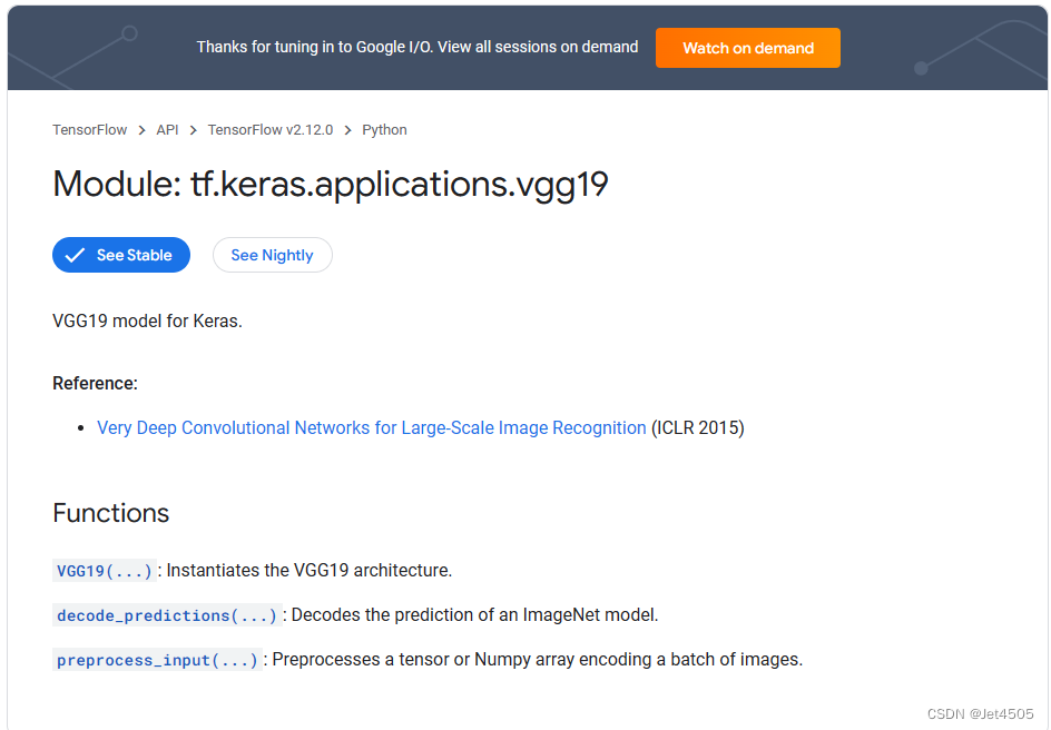
值得注意的是,在Tensorflow 2.X版本的Keras中,已经封装集成了VGG19,因此可以直接调用,还是比较方便的。其实还有一个叫做VGG16,也被集成在Keras中,这里我就不演示了,自行食用。
二、VGG19迁移学习代码实战
我们玩一个有趣的案例:修猫和修狗的识别。其中,修猫5011张,修狗5017张,分别存入单独的文件夹中。
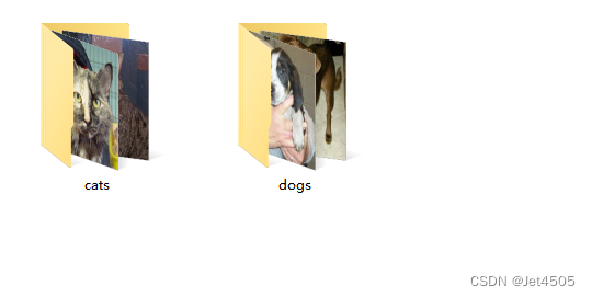
这样,数据就算是准备好了。开始上代码:
(a)导入包
from tensorflow import keras
import tensorflow as tf
from tensorflow.python.keras.layers import Dense, Flatten, Conv2D, MaxPool2D, Dropout, Activation, Reshape, Softmax, GlobalAveragePooling2D
from tensorflow.python.keras.layers.convolutional import Convolution2D, MaxPooling2D
from tensorflow.python.keras import Sequential
from tensorflow.python.keras import Model
from tensorflow.python.keras.optimizers import adam_v2
import numpy as np
import matplotlib.pyplot as plt
from tensorflow.python.keras.preprocessing.image import ImageDataGenerator, image_dataset_from_directory
from tensorflow.python.keras.layers.preprocessing.image_preprocessing import RandomFlip, RandomRotation, RandomContrast, RandomZoom, RandomTranslation
import os,PIL,pathlib
import warnings
#设置GPU
gpus = tf.config.list_physical_devices("GPU")

if gpus:
    gpu0 = gpus[0] #如果有多个GPU,仅使用第0个GPU
    tf.config.experimental.set_memory_growth(gpu0, True) #设置GPU显存用量按需使用
    tf.config.set_visible_devices([gpu0],"GPU")

warnings.filterwarnings("ignore")             #忽略警告信息
plt.rcParams['font.sans-serif'] = ['SimHei']  # 用来正常显示中文标签
plt.rcParams['axes.unicode_minus'] = False    # 用来正常显示负号
(b)导入数据集
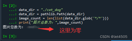
#1.导入数据
data_dir = "./cat_dog"
data_dir = pathlib.Path(data_dir)
image_count = len(list(data_dir.glob('*/*')))
print("图片总数为:",image_count)
batch_size = 16
img_height = 150
img_width = 150
train_ds = image_dataset_from_directory(
data_dir,
validation_split=0.3,
subset="training",
seed=12,
image_size=(img_height, img_width),
batch_size=batch_size)
val_ds = image_dataset_from_directory(
data_dir,
validation_split=0.3,
subset="validation",
seed=12,
image_size=(img_height, img_width),
batch_size=batch_size)
class_names = train_ds.class_names
print(class_names)
#2.检查数据
for image_batch, labels_batch in train_ds:
print(image_batch.shape)
print(labels_batch.shape)
break
#3.配置数据
AUTOTUNE = tf.data.AUTOTUNE
def train_preprocessing(image,label):
return (image/255.0,label)
train_ds = (
train_ds.cache()
.shuffle(1000)
.map(train_preprocessing)
.prefetch(buffer_size=AUTOTUNE)
)
val_ds = (
val_ds.cache()
.shuffle(1000)
.map(train_preprocessing)
.prefetch(buffer_size=AUTOTUNE)
)
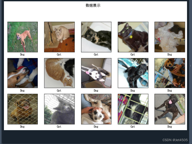
#4. 数据可视化
plt.figure(figsize=(10, 8))
plt.suptitle("数据展示")
class_names = ["Dog","Cat"]
for images, labels in train_ds.take(1):
for i in range(15):
plt.subplot(4, 5, i + 1)
plt.xticks([])
plt.yticks([])
plt.grid(False)
plt.imshow(images[i])
plt.xlabel(class_names[labels[i]-1])
plt.show()输出的图如下:
这里可以调整的是:
①批次(batch_size = 16):也就是一次同时处理多少批次的图片。影响的是计算的速度,依赖的是你的硬件。设置的太高,显卡处理不了,会报错。值得注意的是,批次的设置也会影响后续超参数的调整,所以,最好是先把它固定下来;
②图片的长和宽(img_height = 150,img_width = 150):顾名思义,就是设置丢进模型的图片的分辨率,具体需求也是看你的硬件(RMB);
③验证集的占比(validation_split=0.3):本例中是30%。
再说一个我遇到的坑,关于权限的问题。具体就是导入图片,显示图片为零:
遇事不决,问GPT,回答如下:
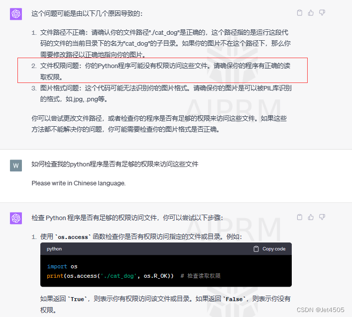
按照TA的提示,我的就是权限问题。因为是直接插的移动硬盘,所以没有给权限。之后我把数据拷贝到电脑,就可以了。
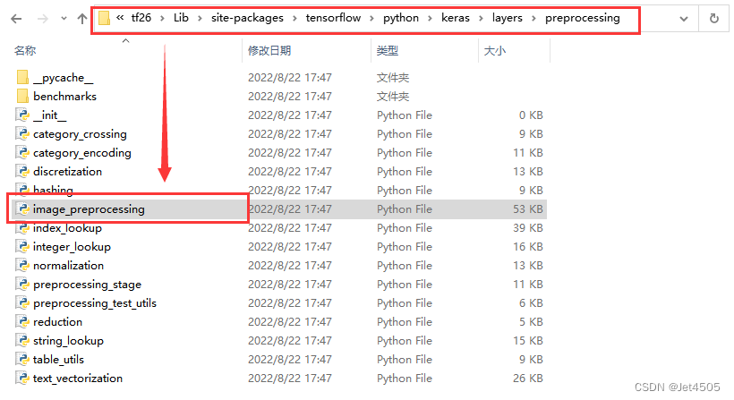
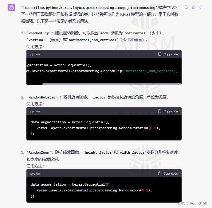
(c)数据增强
data_augmentation = Sequential([
  RandomFlip("horizontal_and_vertical"),
  RandomRotation(0.2),
  #RandomContrast(1.0),
  #RandomZoom(0.5,0.2),
  #RandomTranslation(0.3,0.5),
])

def prepare(ds):
    ds = ds.map(lambda x, y: (data_augmentation(x, training=True), y), num_parallel_calls=AUTOTUNE)
    return ds
train_ds = prepare(train_ds)
可调整的是数据增强的方式。我们可以去下面地址看看内置了哪些数据增强的方式:tensorflow.python.keras.layers.preprocessing.image_preprocessing,还记得怎么找文件夹不?里面有详细解释。
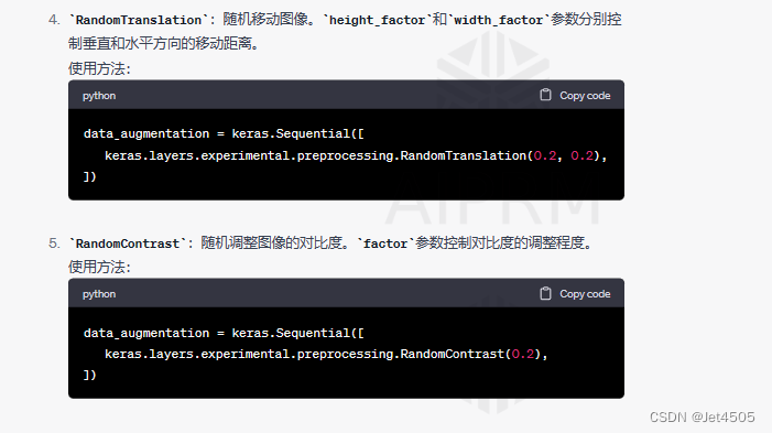
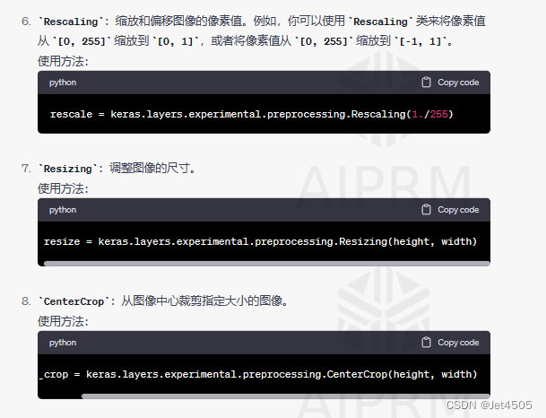
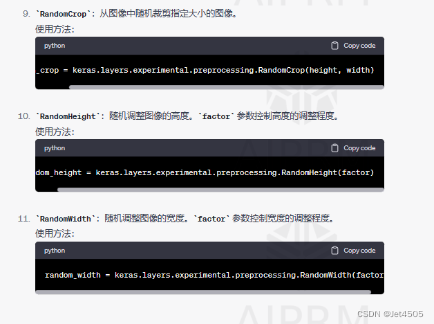
估计你们也不会看,让GPT举几个例子吧:
(d)导入VGG19
#获取预训练模型对输入的预处理方法
from tensorflow.python.keras.applications import vgg19
from tensorflow.python.keras import Input
IMG_SIZE = (img_height, img_width, 3)
base_model = vgg19.VGG19(include_top=False, #是否包含顶层的全连接层
                         weights='imagenet')
#迁移学习主流程代码,开始利用预训练的VGG19创建模型
inputs = Input(shape=IMG_SIZE)
#模型
x = base_model(inputs, training=False) #参数不变化
#全局池化
x = GlobalAveragePooling2D()(x)
#Dropout
x = Dropout(0.3)(x)
#Dense
x = Dense(512, activation='relu')(x)
#输出层
outputs = Dense(2,activation='sigmoid')(x)
#整体封装
model = Model(inputs, outputs)
#打印模型结构
print(model.summary())
这是核心代码,简单解析一下:
这段代码的主要目的是使用预训练的VGG19模型来创建一个新的模型,用于分类任务。下面我会详细解析这段代码:
①导入所需的库:首先,代码从tensorflow.python.keras.applications导入了vgg19模块,这个模块包含了预训练的VGG19模型。然后,从tensorflow.python.keras导入了Input模块,这个模块用于定义模型的输入。
②定义图像大小:IMG_SIZE是一个元组,表示输入图像的大小。这里的img_height和img_width应该在代码的其他部分定义。
③加载预训练的VGG19模型:这里使用vgg19.VGG19函数加载了预训练的VGG19模型。include_top参数设置为False,表示不包含模型的顶层(也就是全连接层)。weights参数设置为'imagenet',表示使用在ImageNet数据集上预训练的权重。
④定义模型的输入:使用Input模块定义了模型的输入,输入的形状是IMG_SIZE。
⑤创建模型:首先,将输入传递给预训练的VGG19模型,得到一个新的输出x。这里的training参数设置为False,表示在这个过程中不更新VGG19模型的参数。然后,使用GlobalAveragePooling2D函数对x进行全局平均池化。接着,使用Dropout函数对x进行dropout操作,dropout率为0.3。然后,使用Dense函数添加一个全连接层,激活函数为relu。最后,使用Dense函数添加一个输出层,激活函数为sigmoid,我们是二分类,所以填入2。
⑥封装模型:使用Model函数将输入和输出封装成一个完整的模型。
然后打印出模型的结构:

(e)编译模型
#定义优化器
from tensorflow.python.keras.optimizers import adam_v2, rmsprop_v2
from tensorflow.python.keras.optimizer_v2.gradient_descent import SGD
optimizer = adam_v2.Adam()
#optimizer = SGD(learning_rate=0.001)
#optimizer = rmsprop_v2.RMSprop()
#编译模型
model.compile(optimizer=optimizer,
                loss='sparse_categorical_crossentropy',
                metrics=['accuracy'])

#训练模型
from tensorflow.python.keras.callbacks import ModelCheckpoint, Callback, EarlyStopping, ReduceLROnPlateau, LearningRateScheduler

NO_EPOCHS = 50
PATIENCE  = 10
VERBOSE   = 1

# 设置动态学习率
annealer = LearningRateScheduler(lambda x: 1e-3 * 0.99 ** (x+NO_EPOCHS))

# 设置早停
earlystopper = EarlyStopping(monitor='loss', patience=PATIENCE, verbose=VERBOSE)

#
checkpointer = ModelCheckpoint('best_model.h5',
                                monitor='val_accuracy',
                                verbose=VERBOSE,
                                save_best_only=True,
                                save_weights_only=True)

train_model  = model.fit(train_ds,
                  epochs=NO_EPOCHS,
                  verbose=1,
                  validation_data=val_ds,
                  callbacks=[earlystopper, checkpointer, annealer])

#保存模型
model.save('JET_VGG19.h5')
print("The trained model has been saved.")
然后,性能悲剧了。迭代了20次,准确率依旧是51%,不能再多了,太难看,我就不放了。接着,求助于GPT,如何改进性能:
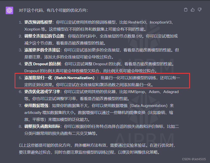
洋洋洒洒列了8项,但是我觉得只有第5项靠谱。接着,问GPT如何改进代码:
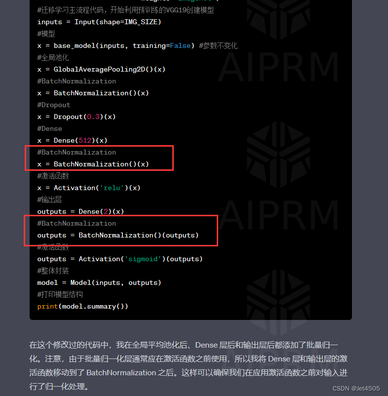
代码如下:
#获取预训练模型对输入的预处理方法
from tensorflow.python.keras.applications import vgg19
from tensorflow.python.keras import Input
IMG_SIZE = (img_height, img_width, 3)
base_model = vgg19.VGG19(include_top=False, #是否包含顶层的全连接层
                         weights='imagenet')

#迁移学习主流程代码,开始利用预训练的VGG19创建模型
inputs = Input(shape=IMG_SIZE)
#模型
x = base_model(inputs, training=False) #参数不变化
#全局池化
x = GlobalAveragePooling2D()(x)
#BatchNormalization
x = BatchNormalization()(x)
#Dropout
x = Dropout(0.3)(x)
#Dense
x = Dense(512)(x)
#BatchNormalization
x = BatchNormalization()(x)
#激活函数
x = Activation('relu')(x)
#输出层
outputs = Dense(2)(x)
#BatchNormalization
outputs = BatchNormalization()(outputs)
#激活函数
outputs = Activation('sigmoid')(outputs)
#整体封装
model = Model(inputs, outputs)
#打印模型结构
print(model.summary())
运行,居然有奇效:
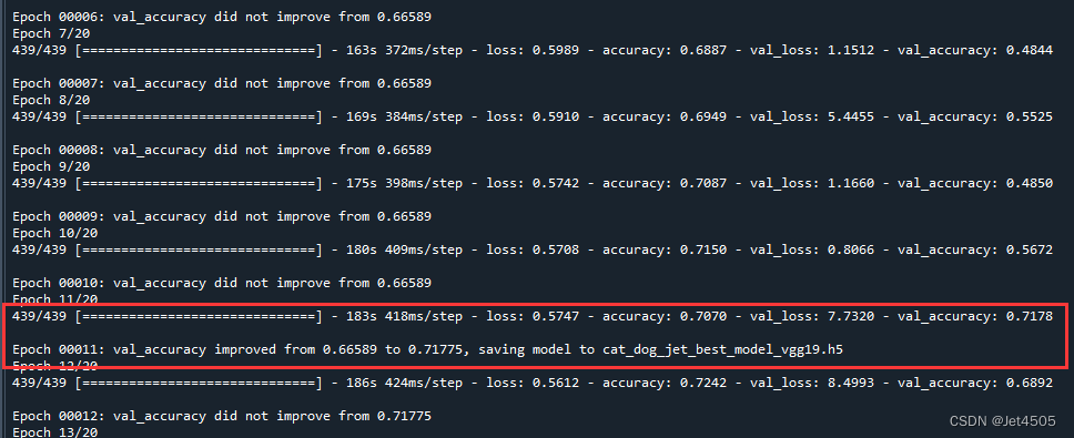
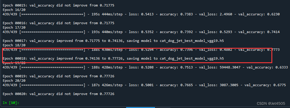
可以看到,迭代到第11次时训练集和验证集的准确率都能达到70%,此时模型被保存为“cat_dog_jet_best_model_vgg19.h5”,方便以后直接调用。因为往后训练有可能性能会变差。当然,如果之后出现性能更好的(例如第18次),会更新最优的模型至“cat_dog_jet_best_model_vgg19.h5”。
(f)Accuracy和Loss可视化
import matplotlib.pyplot as plt

loss = train_model.history['loss']
acc = train_model.history['accuracy']
val_loss = train_model.history['val_loss']
val_acc = train_model.history['val_accuracy']
epoch = range(1, len(loss)+1)

fig, ax = plt.subplots(1, 2, figsize=(10,4))
ax[0].plot(epoch, loss, label='Train loss')
ax[0].plot(epoch, val_loss, label='Validation loss')
ax[0].set_xlabel('Epochs')
ax[0].set_ylabel('Loss')
ax[0].legend()
ax[1].plot(epoch, acc, label='Train acc')
ax[1].plot(epoch, val_acc, label='Validation acc')
ax[1].set_xlabel('Epochs')
ax[1].set_ylabel('Accuracy')
ax[1].legend()
plt.show()
通过这个图,观察模型训练情况:
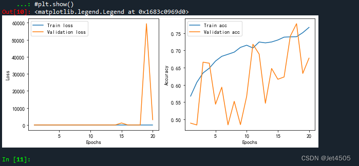
蓝色为训练集,橙色为验证集。
(g)混淆矩阵可视化以及模型参数
没啥好说的,都跟之前的ML模型类似:
import numpy as np
import matplotlib.pyplot as plt
from tensorflow.python.keras.models import load_model
from matplotlib.pyplot import imshow
from sklearn.metrics import classification_report, confusion_matrix
import seaborn as sns
import pandas as pd
import math
# 定义一个绘制混淆矩阵图的函数
def plot_cm(labels, predictions):
# 生成混淆矩阵
conf_numpy = confusion_matrix(labels, predictions)
# 将矩阵转化为 DataFrame
conf_df = pd.DataFrame(conf_numpy, index=class_names ,columns=class_names)
plt.figure(figsize=(8,7))
sns.heatmap(conf_df, annot=True, fmt="d", cmap="BuPu")
plt.title('混淆矩阵',fontsize=15)
plt.ylabel('真实值',fontsize=14)
plt.xlabel('预测值',fontsize=14)
val_pre = []
val_label = []
for images, labels in val_ds:#这里可以取部分验证数据(.take(1))生成混淆矩阵
for image, label in zip(images, labels):
# 需要给图片增加一个维度
img_array = tf.expand_dims(image, 0)
# 使用模型预测图片中的人物
prediction = model.predict(img_array)
val_pre.append(np.argmax(prediction))
val_label.append(label)
plot_cm(val_label, val_pre)
cm_val = confusion_matrix(val_label, val_pre)
a_val = cm_val[0,0]
b_val = cm_val[0,1]
c_val = cm_val[1,0]
d_val = cm_val[1,1]
acc_val = (a_val+d_val)/(a_val+b_val+c_val+d_val) #准确率:就是被分对的样本数除以所有的样本数
error_rate_val = 1 - acc_val #错误率:与准确率相反,描述被分类器错分的比例
sen_val = d_val/(d_val+c_val) #灵敏度:表示的是所有正例中被分对的比例,衡量了分类器对正例的识别能力
sep_val = a_val/(a_val+b_val) #特异度:表示的是所有负例中被分对的比例,衡量了分类器对负例的识别能力
precision_val = d_val/(b_val+d_val) #精确度:表示被分为正例的示例中实际为正例的比例
F1_val = (2*precision_val*sen_val)/(precision_val+sen_val) #F1值:P和R指标有时候会出现的矛盾的情况,这样就需要综合考虑他们,最常见的方法就是F-Measure(又称为F-Score)
MCC_val = (d_val*a_val-b_val*c_val) / (math.sqrt((d_val+b_val)*(d_val+c_val)*(a_val+b_val)*(a_val+c_val))) #马修斯相关系数(Matthews correlation coefficient):当两个类别具有非常不同的大小时,可以使用MCC
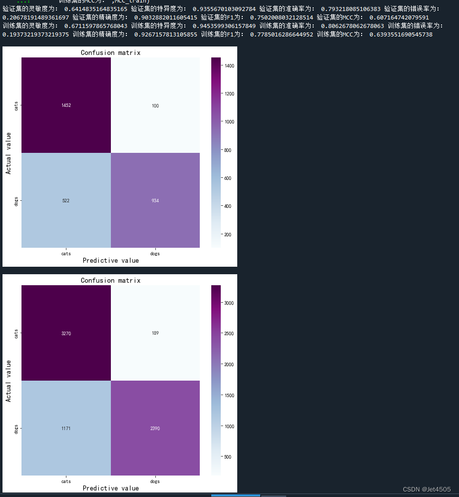
print("验证集的灵敏度为:",sen_val,
"验证集的特异度为:",sep_val,
"验证集的准确率为:",acc_val,
"验证集的错误率为:",error_rate_val,
"验证集的精确度为:",precision_val,
"验证集的F1为:",F1_val,
"验证集的MCC为:",MCC_val)
train_pre = []
train_label = []
for images, labels in train_ds:#这里可以取部分验证数据(.take(1))生成混淆矩阵
for image, label in zip(images, labels):
# 需要给图片增加一个维度
img_array = tf.expand_dims(image, 0)
# 使用模型预测图片中的人物
prediction = model.predict(img_array)
train_pre.append(np.argmax(prediction))
train_label.append(label)
plot_cm(train_label, train_pre)
cm_train = confusion_matrix(train_label, train_pre)
a_train = cm_train[0,0]
b_train = cm_train[0,1]
c_train = cm_train[1,0]
d_train = cm_train[1,1]
acc_train = (a_train+d_train)/(a_train+b_train+c_train+d_train)
error_rate_train = 1 - acc_train
sen_train = d_train/(d_train+c_train)
sep_train = a_train/(a_train+b_train)
precision_train = d_train/(b_train+d_train)
F1_train = (2*precision_train*sen_train)/(precision_train+sen_train)
MCC_train = (d_train*a_train-b_train*c_train) / (math.sqrt((d_train+b_train)*(d_train+c_train)*(a_train+b_train)*(a_train+c_train)))
print("训练集的灵敏度为:",sen_train,
"训练集的特异度为:",sep_train,
"训练集的准确率为:",acc_train,
"训练集的错误率为:",error_rate_train,
"训练集的精确度为:",precision_train,
"训练集的F1为:",F1_train,
"训练集的MCC为:",MCC_train)效果还可以:
AUC值呢,别急,往下看。
(g)AUC曲线绘制
from sklearn import metrics
import numpy as np
import matplotlib.pyplot as plt
from tensorflow.python.keras.models import load_model
from matplotlib.pyplot import imshow
from sklearn.metrics import classification_report, confusion_matrix
import seaborn as sns
import pandas as pd
import math

def plot_roc(name, labels, predictions, **kwargs):
    fp, tp, _ = metrics.roc_curve(labels, predictions)

    plt.plot(fp, tp, label=name, linewidth=2, **kwargs)
    plt.plot([0, 1], [0, 1], color='gray', linestyle='--')
    plt.xlabel('False positives rate')
    plt.ylabel('True positives rate')
    ax = plt.gca()
    ax.set_aspect('equal')

plot_roc("Train Baseline", train_label, train_pre, color="green", linestyle=':')
plot_roc("val Baseline", val_label, val_pre, color="red", linestyle='--')

plt.legend(loc='lower right')

auc_score_train = metrics.roc_auc_score(train_label, train_pre)
auc_score_val = metrics.roc_auc_score(val_label, val_pre)
print("训练集的AUC值为:",auc_score_train, "验证集的AUC值为:",auc_score_val)
输出如下:
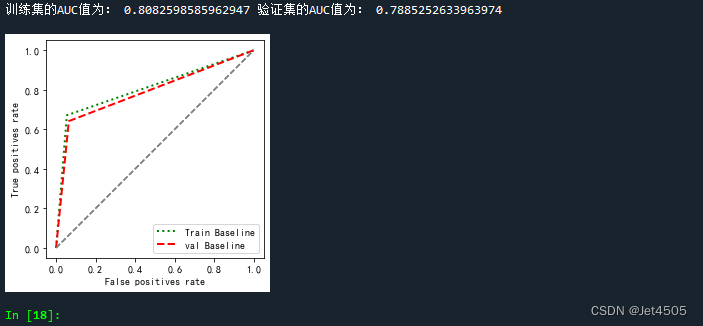
不知道你们发现了没?这个ROC曲线的图有点问题,似乎只有三个点?
这实际上是不准确的,ROC曲线应该反映的是不同的阈值所对应的灵敏度和特异度的数值,所以不应该只有三个点。那么需要怎么修改呢?代码如下:
from sklearn import metrics
import numpy as np
import matplotlib.pyplot as plt
from tensorflow.python.keras.models import load_model
from matplotlib.pyplot import imshow
from sklearn.metrics import classification_report, confusion_matrix
import seaborn as sns
import pandas as pd
import math
def plot_roc(name, labels, predictions, **kwargs):
fp, tp, _ = metrics.roc_curve(labels, predictions)
plt.plot(fp, tp, label=name, linewidth=2, **kwargs)
plt.plot([0, 1], [0, 1], color='orange', linestyle='--')
plt.xlabel('False positives rate')
plt.ylabel('True positives rate')
ax = plt.gca()
ax.set_aspect('equal')
val_pre_auc = []
val_label_auc = []
for images, labels in val_ds:
for image, label in zip(images, labels):
img_array = tf.expand_dims(image, 0)
prediction_auc = model.predict(img_array)
val_pre_auc.append((prediction_auc)[:,1])
val_label_auc.append(label)
auc_score_val = metrics.roc_auc_score(val_label_auc, val_pre_auc)
train_pre_auc = []
train_label_auc = []
for images, labels in train_ds:
for image, label in zip(images, labels):
img_array_train = tf.expand_dims(image, 0)
prediction_auc = model.predict(img_array_train)
train_pre_auc.append((prediction_auc)[:,1])#输出概率而不是标签!
train_label_auc.append(label)
auc_score_train = metrics.roc_auc_score(train_label_auc, train_pre_auc)
plot_roc('validation AUC: {0:.4f}'.format(auc_score_val), val_label_auc , val_pre_auc , color="red", linestyle='--')
plot_roc('training AUC: {0:.4f}'.format(auc_score_train), train_label_auc, train_pre_auc, color="blue", linestyle='--')
plt.legend(loc='lower right')
#plt.savefig("roc.pdf", dpi=300,format="pdf")
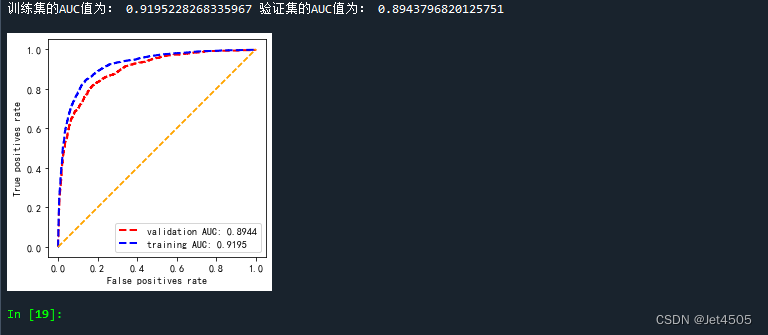
print("训练集的AUC值为:",auc_score_train, "验证集的AUC值为:",auc_score_val)关键在于:
train_pre_auc.append((prediction_auc)[:,1]),以及val_pre_auc.append((prediction_auc)[:,1]),输出的是概率而不是标签(0或者1)!
三、测试模型
既然构建了模型,那么就得拿来试一试自家的修猫:
#保存模型
model.save('cat_dog_jet_best_model_vgg19.h5')
print("The trained model has been saved.")

#测试模型
from tensorflow.python.keras.models import load_model
from tensorflow.python.keras.preprocessing import image
from tensorflow.python.keras.preprocessing.image import img_to_array
from PIL import Image
import os, shutil, pathlib
label=np.array(["Dog","Cat"])#0、1赋值给标签
#载入模型
model=load_model('cat_dog_jet_best_model_vgg19.h5.h5')
#导入图片
image=image.load_img('E:/ML/Deep Learning/laola.jpg')#手动修改路径,删除隐藏字符
plt.imshow(image)
plt.show()
image=image.resize((img_width,img_height))
image=img_to_array(image)
image=image/255#数值归一化,转为0-1
image=np.expand_dims(image,0)
print(image.shape)
# 使用模型进行预测
predictions = model.predict(image)
predicted_class = np.argmax(predictions)
# 打印预测的类别
print(label[predicted_class])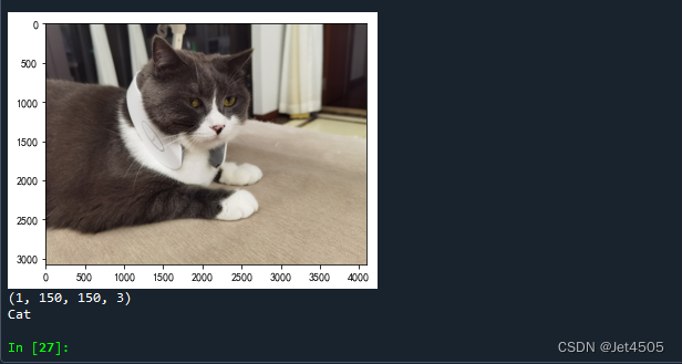
至少是一只猫,虽然有狗的灵魂。
四、数据
链接:https://pan.baidu.com/s/1iPiKFaMbIPwKC-dgkChO3w?pwd=y6c9
提取码:y6c9