文章目录
- 神经网络基本原理
- 线性分类器
- 学习率
- 一个线性分类器的局限性
- 逻辑AND、逻辑OR
- 逻辑XOR
- 神经元
- sigmoid function的logistic function(逻辑函数)
- 多层神经元
- 演示只有两层,每层两个神经元的神经网络的工作
- 矩阵大法(点乘)
- 使用矩阵乘法的三层神经网络示例
- 反向传播误差
- 多个输出节点反向传播误差
- 使用矩阵乘法进行反向传播误差
- 更新权重
- 梯度下降法
- 误差函数
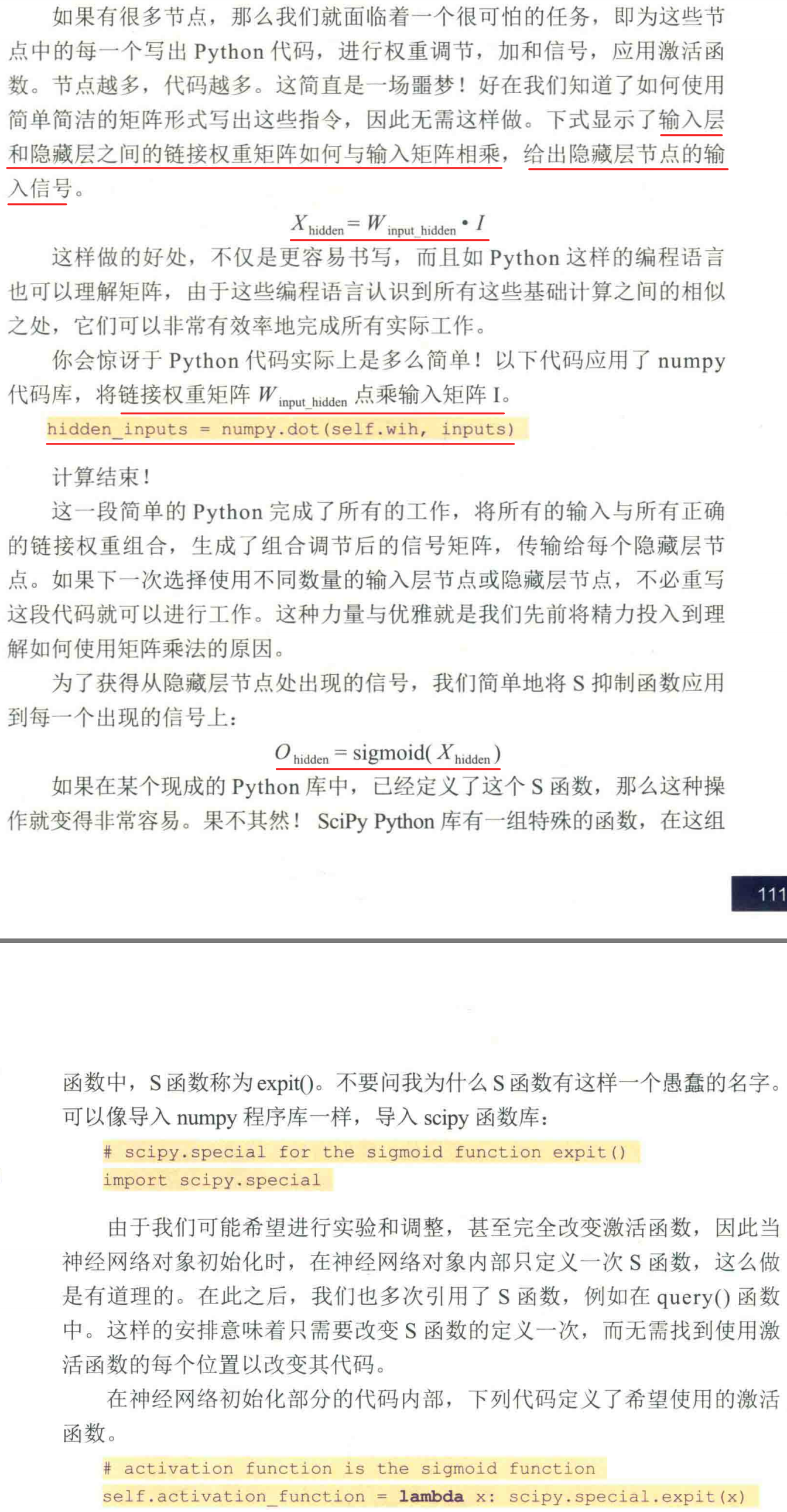
- 激活函数sigmoid
- Python相关知识回顾
- 数组
- 绘制数组
- 对象
- 使用Python制作神经网络
- 框架代码
- 初始化网络
- 权重——网络的核心
- 查询网络
- 训练网络
- 目前为止的代码
- 实战——使用手写数字的数据集MNIST测试神经网络
- 准备MNIST训练数据
- 使用部分数据集测试网络
- 使用完整数据集进行训练和测试
- 一些改进:调整学习率
- 一些改进:训练多世代
- 改变网络形状
- 测试自己的手写数字
- 神经网络黑盒子
- 向后查询
- 利用现有神经网络反向输出图像
- 创建新的训练数据:旋转图像
- scipy.ndimage.rotate
- 旋转数据集“1”
- 添加旋转图像数据集进行神经网络的训练和测试
- 想获取更多神经网络深度学习强化学习资料可以私信我。之后我会持续更新,如果喜欢我的文章,请记得一键三连哦,点赞关注收藏,你的每一个赞每一份关注每一次收藏都将是我前进路上的无限动力 !!!↖(▔▽▔)↗感谢支持!
神经网络基本原理
用来训练预测器或分类器的真实实例,我们称为训练数据。
误差值E =(期望目标值 - 实际输出值)
线性分类器

学习率


一个线性分类器的局限性
布尔逻辑函数通常需要两个输入,并输出一个答案

逻辑AND、逻辑OR
计算机通常使用数字1表示真,使用数字0表示假


逻辑XOR


神经元

观察表明,神经元不会立即反应,而是会抑制输入,直到输入增强,强大到可以触发输出。你可以这样认为,在产生输出之前,输入必须到达一个阈值。就像水在杯中—直到水装满了杯子,才可能溢出。直观上,这是有道理的—神经元不希望传递微小的噪声信号,而只是传递有意识的明显信号。下图说明了这种思想,只有输入超过了阈值(threshold),足够接通电路,才会产生输出信号。

虽然这个函数接受了输入信号,产生了输出信号,但是我们要将某种称为激活函数的阈值考虑在内。在数学上,有许多激活函数可以达到这样的效果。一个简单的阶跃函数可以实现这种效果

你可以看到,在输入值较小的情况下,输出为零。然而,一旦输入达到阈值,输出就一跃而起。具有这种行为的人工神经元就像一个真正的生物神经元。科学家所使用的术语实际上非常形象地描述了这种行为,他们说,输入达到阈值时,神经元就激发了
sigmoid function的logistic function(逻辑函数)
A.K.A scipy.special.expit


我们要认识到的第一件事情是生物神经元可以接受许多输入,而不仅仅是一个输入。刚才,我们观察了布尔逻辑机器有两个输入,因此,有多个输入的想法并不新鲜,并非不同寻常。
对于所有这些输入,我们该做些什么呢?我们只需对它们进行相加,得到最终总和,作为S函数的输入,然后输出结果。这实际上反映了神经元的工作机制。下图说明了这种组合输入,然后对最终输入总和使用阈值的思路

需要注意的一点是,每个神经元接受来自其之前多个神经元的输入,并且如果神经元被激发了,它也同时提供信号给更多的神经元。
多层神经元
将这种自然形式复制到人造模型的一种方法是,构建多层神经元,每一层中的神经元都与在其前后层的神经元互相连接。下图详细描述了这种思想


你可能有充分的理由来挑战这种设计,质问为什么必须把前后层的每一个神经元与所有其他层的神经元互相连接,并且你甚至可以提出各种创造性的方式将这些神经元连接起来。我们不采用创造性的方式将神经元连接起来,原因有两点,第一是这种一致的完全连接形式事实上可以相对容易地编码成计算机指令,第二是神经网络的学习过程将会弱化这些实际上不需要的连接(也就是这些连接的权重将趋近于0),因此对于解决特定任务所需最小数量的连接冗余几个连接,也无伤大雅。


演示只有两层,每层两个神经元的神经网络的工作
尝试使用只有两层、每层两个神经元的较小的神经网络,来演示神经网络如何工作


第一层节点是输入层,这一层不做其他事情,仅表示输入信号。也就是说,输入节点不对输入值应用激活函数。这没有什么其他奇妙的原因,自然而然地,历史就是这样规定的。神经网络的第一层是输入层,这层所做的所有事情就是表示输入,仅此而已


矩阵大法(点乘)
在一些书中,你会看到这样的矩阵乘法称为点乘(dot product)或内积(inner product)。实际上,对于矩阵而言,有不同类型的乘法,如叉乘,但是我们此处所指的是点乘


使用矩阵乘法的三层神经网络示例


需要记住的事情是,不管有多少层神经网络,我们都“一视同仁”,即组合输入信号,应用链接权重调节这些输入信号,应用激活函数,生成这些层的输出信号。我们不在乎是在计算第3层、第53层或是第103层的信号,使用的方法如出一辙。


反向传播误差
先前,我们通过调整节点线性函数的斜率参数,来调整简单的线性分类器。我们使用误差值,也就是节点生成了答案与所知正确答案之间的差值,引导我们进行调整。实践证明,误差与所必须进行的斜率调整量之间的关系非常简单,调整过程非常容易。
当输出和误差是多个节点共同作用的结果时,我们如何更新链接权重呢?下图详细阐释了这个问题。

多个输出节点反向传播误差

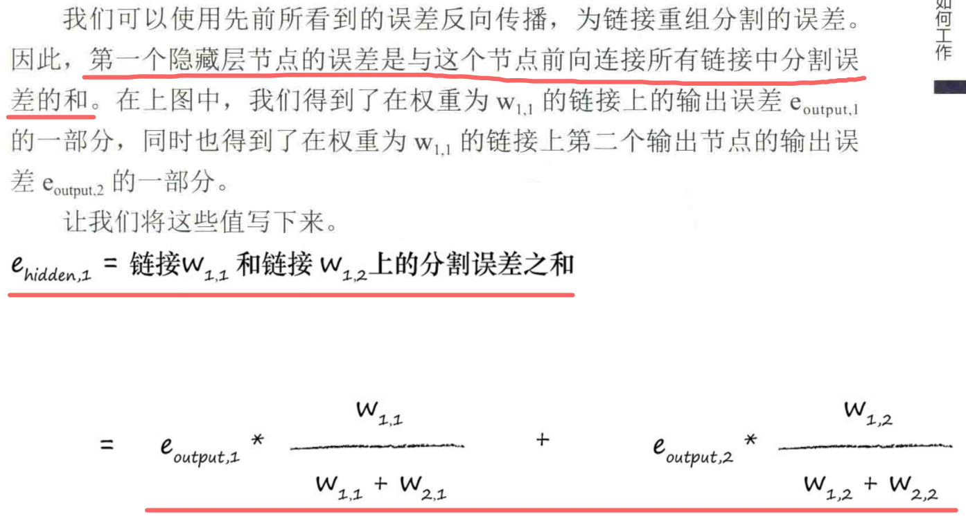
两个输出节点都有误差—事实上,在未受过训练的神经网络中,这是极有可能发生的情况。你会发现,在网络中,我们需要使用这两个误差值来告知如何调整内部链接权重。我们可以使用与先前一样的方法,也就是跨越造成误差的多条链接,按照权重比例,分割输出节点的误差。


如果神经网络具有多个层,那么我们就从最终输出层往回工作,对每一层重复应用相同的思路。误差信息流具有直观意义。同样,你明白为什么我们称之为误差的反向传播了。


如下图所示,我们进一步向后工作,在前一层中应用相同的思路


使用矩阵乘法进行反向传播误差
计算的起始点是在神经网络最终输出层中出现的误差。此时,在输出层,神经网络只有两个节点,因此误差只有e1和e2


更新权重
到目前为止,我们已经理解了让误差反向传播到网络的每一层。为什么这样做呢?原因就是,我们使用误差来指导如何调整链接权重,从而改进神经网络输出的总体答案。
但是,这些节点都不是简单的线性分类器。这些稍微复杂的节点,对加权后的信号进行求和,并应用了S阈值函数,将所得到的结果输出给下一层的节点。

梯度下降法
在数学上,这种方法称为梯度下降(gradient descent),你可以明白这是为什么吧。在你迈出一步之后,再次观察周围的地形,看看你下一步往哪个方向走,才能更接近目标,然后,你就往那个方向走出一步。你一直保持这种方式,直到非常欣喜地到达了山底。梯度是指地面的坡度。你走的方向是最陡的坡度向下的方向。

现在,想象一下,这个复杂的地形是一个数学函数。梯度下降法给我们带来一种能力,即我们不必完全理解复杂的函数,从数学上对函数进行求解,就可以找到最小值。如果函数非常困难,我们不能用代数轻松找到最小值,我们就可以使用这个方法来代替代数方法。
当然,由于我们采用步进的方式接近答案,一点一点地改进所在的位置,因此这可能无法给出精确解。但是,这比得不到答案要好。总之,我们可以使用更小的步子朝着实际的最小值方向迈进,优化答案,直到我们对于所得到的精度感到满意为止。
这种酷炫的梯度下降法与神经网络之间有什么联系呢?好吧,如果我们将复杂困难的函数当作网络误差,那么下山找到最小值就意味着最小化误差。这样我们就可以改进网络输出。这就是我们希望做到的!


误差函数


现在,我们需要完成工作,为输入层和隐藏层之间的权重找到类似的误差斜率。


激活函数sigmoid
仔细观察下图的S激活函数。你可以发现,如果输入变大,激活函数就会变得非常平坦

权重的改变取决于激活函数的梯度。小梯度意味着限制神经网络学习的能力。这就是所谓的饱和神经网络。这意味着,我们应该尽量保持小的输入。

神经网络的输出是最后一层节点弹出的信号。如果我们使用的激活函数不能生成大于1的值,那么尝试将训练目标值设置为比较大的值就有点愚蠢了。请记住,逻辑函数甚至不能取到1.0,只能接近1.0。数学家称之为渐近于1.0。


Python相关知识回顾
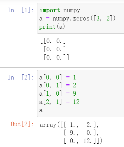
数组
绘制数组
绘制二维数字数组的一种方式是将它们视为二维平面,根据数组中单元格的值对单元格进行着色。你可以选择如何将单元格中的某个数值转换为某种色彩。
你可以简单地选择根据颜色标度,将数值转换为某种颜色,或者将超过某一阈值的单元格涂上黑色,剩余其他的一切单元格都涂为白色。


对象
我们再来学习一个Python的思想,即对象。由于我们只定义对象一次,却可以多次使用对象,因此对象类似于可重用函数。但是,比起简单的函数,对象可以做的事情要多得多。
class Dog:
    def bark(self):
        print("woof!")
        pass
    pass
让我们从熟悉的内容开始。你可以看到,在代码内有一个函数名为bark()。如果我们调用这个函数,就很容易看到这个动作,即在屏幕上打印出了“woof! ”。
现在,让我们来看看这个熟悉的函数定义。你可以看到关键字class、名字“Dog”和一个看起来像函数的结构。这与函数的定义相似,也有一个名字。不同之处在于,函数使用关键字“def”来定义,而这里使用“class”来定义对象。


你可能已经发现了函数定义bark(self)中的“self”。这似乎很奇怪,我对此也感到很奇怪。我非常喜欢Python,但是我并不认为Python是完美的。“self”之所以出现在那里,是为了当Python创建函数时,Python能将函数赋予正确的对象。但是我个人的看法是:由于bark()是在类定义的内部,因此Python应该知道这个函数连接到了哪个对象,这是显而易见的。


class Dog:
    def __init__(self, petname, temp):
        self.name = petname;
        self.temperature = temp;

    def status(self):
        print("dog name is ", self.name)
        print("dog temperature is ", self.temperature)
        pass

    def setTemperature(self, temp):
        self.temperature = temp;
        pass

    def bark(self):
        print("woof!")
        pass

    pass
首先要注意的事情是,我们添加了3个新函数到Dog类中。我们已经有了bark()函数,现在又有了新的函数,名为__init __()、status()和setTemperature()。很容易理解添加新函数。如果愿意,也可以添加名为sneeze()的新函数与bark()匹配。

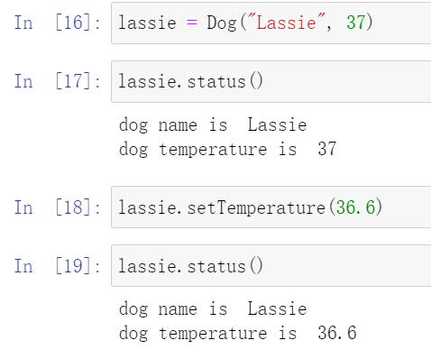
下图显示了使用这些新函数定义的新Dog类以及名为lassie的新的Dog对象,我们使用参数将其命名为“Lassie”,设置初始温度为37,创建了这个对象。
使用Python制作神经网络
框架代码

所编写的代码框架如下所示:
# neural network class definition
class neuralNetwork:
    # initialise the neural network
    def __init__():
        pass

    # train the neural network
    def train():
        pass

    # query the neural network
    def query():
        pass
初始化网络
从初始化网络开始。我们需要设置输入层节点、隐藏层节点和输出层节点的数量。这些节点数量定义了神经网络的形状和尺寸。我们不会将这些数量固定,而是当我们使用参数创建一个新的神经网络对象时,才会确定这些数量。通过这种方式,我们保留了选择的余地,轻松地创建不同大小的新神经网络。
# neural network class definition
class neuralNetwork:
    # initialise the neural network
    def __init__(self, inputnodes, hiddennodes, outputnodes, learningrate):
        # set number of nodes in each input, hidden, output layer
        self.inodes = inputnodes
        self.hnodes = hiddennodes
        self.onodes = outputnodes

        # learning rate
        self.lr = learningrate

        pass

    # train the neural network
    def train():
        pass

    # query the neural network
    def query():
        pass
让我们使用所定义的神经网络类,尝试创建每层3个节点、学习率为0.5的小型神经网络对象。
# number of input, hidden and output nodes
input_nodes = 3
hidden_nodes = 3
output_nodes = 3

# learning rate is 0.3
learning_rate = 0.3

# create instance of neural network
n = neuralNetwork(input_nodes,hidden_nodes,output_nodes, learning_rate)
权重——网络的核心
下一步是创建网络的节点和链接。网络中最重要的部分是链接权重,我们使用这些权重来计算前馈信号、反向传播误差,并且在试图改进网络时优化链接权重本身

# link weight matrices, wih and who
# weights inside the arrays are w_i_j, where link is from node i to node j in the next
# layer
# w11 w21 w12 w22 etc
self.wih = (numpy.random.rand(self.hnodes, self.inodes) - 0.5)
self.who = (numpy.random.rand(self.onodes, self.hnodes) - 0.5)


# 从正态(高斯)分布中抽取随机样本构建权重矩阵
# numpy.random.normal(mean, std, size)
# pow(self.hnodes, -0.5)和pow(self.onodes, -0.5)是经验规则
# 数学家所得到的经验规则是,我们可以在一个节点传入链接数量平方根倒数的大致范围内随机采样,初始化权重。
self.wih = numpy.random.normal(0.0, pow(self.hnodes, -0.5), (self.hnodes, self.inodes))
self.who = numpy.random.normal(0.0, pow(self.onodes, -0.5), (self.onodes, self.hnodes))
我们将正态分布的中心设定为0.0。与下一层中节点相关的标准方差的表达式,按照Python的形式,就是pow(self.hnodes,-0.5),简单说来,这个表达式就是表示节点数目的-0.5次方。最后一个参数,就是我们希望的numpy数组的形状大小。
查询网络
query()函数接受神经网络的输入,返回网络的输出。这个功能非常简单,但是,为了做到这一点,你要记住,我们需要传递来自输入层节点的输入信号,通过隐藏层,最后从输出层输出。你还要记住,当信号馈送至给定的隐藏层节点或输出层节点时,我们使用链接权重调节信号,还应用S激活函数抑制来自这些节点的信号。

# neural network class definition
class neuralNetwork:
    # initialise the neural network
    def __init__(self, inputnodes, hiddennodes, outputnodes, learningrate):
        # set number of nodes in each input, hidden, output layer
        self.inodes = inputnodes
        self.hnodes = hiddennodes
        self.onodes = outputnodes

        # link weight matrices, wih and who
        # weights inside the arrays are w_i_j, where link is from node i to node j in the next
        # layer
        # w11 w21 w12 w22 etc
        # self.wih = (numpy.random.rand(self.hnodes, self.inodes) - 0.5)
        # self.who = (numpy.random.rand(self.onodes, self.hnodes) - 0.5)
        # 从正态(高斯)分布中抽取随机样本构建权重矩阵
        # numpy.random.normal(mean, std, size)
        # pow(self.hnodes, -0.5)和pow(self.onodes, -0.5)是经验规则
        # 数学家所得到的经验规则是,我们可以在一个节点传入链接数量平方根倒数的大致范围内随机采样,初始化权重。
        self.wih = numpy.random.normal(0.0, pow(self.hnodes, -0.5), (self.hnodes, self.inodes))
        self.who = numpy.random.normal(0.0, pow(self.onodes, -0.5), (self.onodes, self.hnodes))

        # 学习率
        self.lr = learningrate

        # activation function is the sigmoid function
        # 激活函数
        self.activation_function = lambda x: scipy.special.expit(x)
        pass

    # train the neural network
    def train():
        pass

    # query the neural network
    def query(self, inputs_list):
        # convert inputs list to 2d array
        # 把输入值转化为列向量
        inputs = numpy.array(inputs_list, ndmin=2).T

        # calculate signals into hidden layer
        hidden_inputs = numpy.dot(self.wih, inputs)
        # calculate the signals emerging from hidden layer
        hidden_outputs = self.activation_function(hidden_inputs)

        # calculate signals into output layer
        final_inputs = numpy.dot(self.who, hidden_outputs)
        # calculate the signals emerging from final output layer
        final_outputs = self.activation_function(final_inputs)
        return final_outputs
# number of input, hidden and output nodes
input_nodes = 3
hidden_nodes = 3
output_nodes = 3

# learning rate is 0.3
learning_rate = 0.3

# create instance of neural network
n = neuralNetwork(input_nodes, hidden_nodes, output_nodes, learning_rate)

n.query([1.0, 0.5, -1.5])

训练网络
训练任务分为两个部分:

# train the neural network
def train(self, inputs_list, targets_list):
	# convert inputs list to 2d array
    # 把输入值转化为列向量
    inputs = numpy.array(inputs_list, ndmin=2).T
    # 把目标输出值转化为列向量
    targets = numpy.array(targets_list, ndmin=2).T

    # calculate signals into hidden layer
    hidden_inputs = numpy.dot(self.wih, inputs)
    # calculate the signals emerging from hidden layer
    hidden_outputs = self.activation_function(hidden_inputs)

    # calculate signals into output layer
    final_inputs = numpy.dot(self.who, hidden_outputs)
    # calculate the signals emerging from final output layer
    final_outputs = self.activation_function(final_inputs)

    pass

目前为止的代码
import numpy
# scipy.special for the sigmoid function expit()
import scipy.special

# neural network class definition
class neuralNetwork:
    # initialise the neural network
    def __init__(self, inputnodes, hiddennodes, outputnodes, learningrate):
        # set number of nodes in each input, hidden, output layer
        self.inodes = inputnodes
        self.hnodes = hiddennodes
        self.onodes = outputnodes

        # link weight matrices, wih and who
        # weights inside the arrays are w_i_j, where link is from node i to node j in the next
        # layer
        # w11 w21 w12 w22 etc
        # self.wih = (numpy.random.rand(self.hnodes, self.inodes) - 0.5)
        # self.who = (numpy.random.rand(self.onodes, self.hnodes) - 0.5)
        # 从正态(高斯)分布中抽取随机样本构建权重矩阵
        # numpy.random.normal(mean, std, size)
        # pow(self.hnodes, -0.5)和pow(self.onodes, -0.5)是经验规则
        # 数学家所得到的经验规则是,我们可以在一个节点传入链接数量平方根倒数的大致范围内随机采样,初始化权重。
        self.wih = numpy.random.normal(0.0, pow(self.hnodes, -0.5), (self.hnodes, self.inodes))
        self.who = numpy.random.normal(0.0, pow(self.onodes, -0.5), (self.onodes, self.hnodes))

        # 学习率
        self.lr = learningrate

        # activation function is the sigmoid function
        # 激活函数
        self.activation_function = lambda x: scipy.special.expit(x)
        pass

    # train the neural network
    def train(self, inputs_list, targets_list):
        # convert inputs list to 2d array
        # 把输入值转化为列向量
        inputs = numpy.array(inputs_list, ndmin=2).T
        # 把目标输出值转化为列向量
        targets = numpy.array(targets_list, ndmin=2).T

        # calculate signals into hidden layer
        hidden_inputs = numpy.dot(self.wih, inputs)
        # calculate the signals emerging from hidden layer
        hidden_outputs = self.activation_function(hidden_inputs)

        # calculate signals into output layer
        final_inputs = numpy.dot(self.who, hidden_outputs)
        # calculate the signals emerging from final output layer
        final_outputs = self.activation_function(final_inputs)

        # output layer error is the (target - actual)
        output_errors = targets - final_outputs
        # hidden layer error is the output_errors, split by weights, recombined at hidden nodes
        hidden_errors = numpy.dot(self.who.T, output_errors)

        # update the weights for the links between the hidden and output layers
        # 更新隐藏层到输出层的权重
        self.who += self.lr * numpy.dot((output_errors * final_outputs * (1.0 - final_outputs)), numpy.transpose(hidden_outputs))
        # update the weights for the links between the input and hidden layers
        # 更新输入层到隐藏层的权重
        self.wih += self.lr * numpy.dot((hidden_errors * hidden_outputs * (1.0 - hidden_outputs)), numpy.transpose(inputs))
        pass

    # query the neural network
    def query(self, inputs_list):
        # convert inputs list to 2d array
        # 把输入值转化为列向量
        inputs = numpy.array(inputs_list, ndmin=2).T
        # print(inputs)

        # calculate signals into hidden layer
        hidden_inputs = numpy.dot(self.wih, inputs)
        # calculate the signals emerging from hidden layer
        hidden_outputs = self.activation_function(hidden_inputs)

        # calculate signals into output layer
        final_inputs = numpy.dot(self.who, hidden_outputs)
        # calculate the signals emerging from final output layer
        final_outputs = self.activation_function(final_inputs)
        return final_outputs
实战——使用手写数字的数据集MNIST测试神经网络
这个数据集称为手写数字的MNIST数据库。从受人尊敬的神经网络研究员Yann LeCun的网站http://yann.lecun.com/exdb/mnist/,可以得到这个数据集。
这个网页也列出了在学习和正确识别这些手写字符方面,这些新旧想法的表现如何。我们将会多次提到这个列表,看看比起专业人士我们的想法表现如何!MNIST数据库的格式不容易使用,因此其他人已经创建了相对简单的数据文件格式,参见http://pjreddie.com/projects/mnist-in-csv/,这对我们非常有帮助。
这些文件称为CSV文件,这意味着纯文本中的每一个值都是由逗号分隔的。你可以轻松地在任何文本编辑器中查看这些数值,大部分的电子表格和数据分析软件也兼容CSV文件,它们是非常通用的标准。
这个网站提供了两个CSV文件:
· 训练集http://www.pjreddie.com/media/files/mnist_train.csv
· 测试集http://www.pjreddie.com/media/files/mnist_test.csv
顾名思义,训练集是用来训练神经网络的60000个标记样本集。标记是指输入与期望的输出匹配,也就是答案应该是多少

在文本中,这些记录或这些行的内容很容易理解:
· 第一个值是标签,即书写者实际希望表示的数字,如“7”或“9”。这是我们希望神经网络学习得到的正确答案。
· 随后的值,由逗号分隔,是手写体数字的像素值。像素数组的尺寸是28乘以28,因此在标签后有784个值。
在深入研究进行这样操作之前,我们应该下载MNIST数据集中的一个较小的子集。MNIST数据的数据文件是相当大的,而较小的子集意味着我们可以实验、尝试和开发代码,而不会由于大量的数据集而拖慢计算机的速度,因此小数据集还是大有裨益的。一旦确定了乐于使用的算法和代码,我们就可以使用完整的数据集。
以下是MNIST数据集中较小子集的链接,也是以CSV格式存储的:
· MNIST测试数据集中的10条记录 https://raw.githubusercontent.com/makeyourownneuralnetwork/makeyourownneuralnetwork/master/mnist_dataset/mnist_test_10.csv
· MNIST训练数据集中的100条记录 https://raw.githubusercontent.com/makeyourownneuralnetwork/makeyourownneuralnetwork/master/mnist_dataset/mnist_train_100.csv
文件存放目录树


data_file = open("mnist_dataset/mnist_train_100.csv", 'r')
data_list = data_file.readlines()
data_file.close()
第一行使用open()函数打开一个文件。传递给函数的第一个参数是文件的名称。其实,这不仅仅是文件名“mnist_train_100.csv”,这是整个路径,其中包括了文件所在的目录。第二个参数是可选的,它只是告诉Python我们希望如何处理文件。“r”告诉Python以只读的方式而不是可写的方式打开文件。这样可以避免任何更改数据或删除数据的意外。如果试图写入文件、修改文件,Python将阻止并生成一条错误消息。


准备MNIST训练数据
我们已经知道如何获取和折开MNIST数据文件中的数据,从而理解并可视化这些数据。我们要使用此数据训练神经网络,但是我们需要想想,在将数据抛给神经网络之前如何准备数据。
我们需要做的第一件事情是将输入颜色值从较大的0到255的范围,缩放至较小的0.01 到1.0的范围。我们刻意选择0.01作为范围最低点,是为了避免先前观察到的0值输入最终会人为地造成权重更新失败。我们没有选择0.99作为输入的上限值,是因为不需要避免输入1.0会造成这个问题。我们只需要避免输出值为1.0。
将在0到255范围内的原始输入值除以255,就可以得到0到1范围的输入值。然后,需要将所得到的输入乘以0.99,把它们的范围变成0.0到0.99。接下来,加上0.01,将这些值整体偏移到所需的范围0.01到1.00。
scaled_input = (numpy.asfarray(all_values[1:]) / 255.0 * 0.99) + 0.01
print(scaled_input)
但是,实际上,我们要问自己一个更深层次的问题。输出应该是什么样子的?这应该是图片答案吗?这意味着有28×28=784个输出节点。
如果退后一步,想想要求神经网络做什么,我们会意识到,要求神经网络对图像进行分类,分配正确的标签。这些标签是0到9共10个数字中的一个。这意味着神经网络应该有10个输出层节点,每个节点对应一个可能的答案或标签。如果答案是“0”,输出层第一个节点激发,而其余的输出节点则保持抑制状态。如果答案是“9”,输出层的最后节点会激发,而其余的输出节点则保持抑制状态。下图详细阐释了这个方案,并显示了一些示例输出

第一个示例是神经网络认为它看到的是数字“5”。可以看到,从输出层出现的最大信号来自于标签为5的节点。由于从标签0开始,因此这是第六个节点。这很容易吧。其余的输出节点产生的信号非常小,接近于零。舍入误差可能导致零输出,但事实上,要记住激活函数不会产生实际为零的输出。
下一个示例演示了如果神经网络认为它看到了手写的“0”将会发生的事情。同样,目前最大输出来自于第一个输出节点,对应的标签为“0”。
最后一个示例更有趣。这里,神经网络的最大输出信号来自于最后一个节点,对应标签“9”。然而,在标签为“4”的节点处,它得到了中等大小的输出。通常,我们会使用最大信号为答案,但是,可以看看网络为何会认为答案可能是“4”。也许笔迹使得它难以确定?神经网络中确实会发生这种不确定性,我们不应该把它看作是一件坏事,而应该将其视为有用的见解,即另一个答案也可能满足条件。
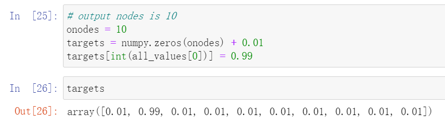
如果训练样本的标签为“5”,那么需要创建输出节点的目标数组,其中除了对应于标签“5”的节点,其他所有节点的值应该都很小,这个数组看起来可能如[0, 0, 0, 0, 0, 1, 0, 0, 0, 0]。
事实上,我们已经明白了,试图让神经网络生成0和1的输出,对于激活函数而言是不可能的,这会导致大的权重和饱和网络,因此需要重新调整这些数字。我们将使用值0.01和0.99来代替0和1,这样标签为“5”的目标输出数组为[0.01, 0.01,0.01, 0.01, 0.01, 0.99, 0.01, 0.01, 0.01, 0.01]
# output nodes is 10
onodes = 10
targets = numpy.zeros(onodes) + 0.01
targets[int(all_values[0])] = 0.99
import numpy
# scipy.special for the sigmoid function expit()
import scipy.special
# library for plotting arrays
import matplotlib.pyplot
# ensure the plots are inside this notebook, not an external window
%matplotlib inline

# neural network class definition
# code for a 3-layer neural network, and code for learning the MNIST dataset
class neuralNetwork:
    # initialise the neural network
    def __init__(self, inputnodes, hiddennodes, outputnodes, learningrate):
        # set number of nodes in each input, hidden, output layer
        self.inodes = inputnodes
        self.hnodes = hiddennodes
        self.onodes = outputnodes

        # link weight matrices, wih and who
        # weights inside the arrays are w_i_j, where link is from node i to node j in the next
        # layer
        # w11 w21 w12 w22 etc
        # self.wih = (numpy.random.rand(self.hnodes, self.inodes) - 0.5)
        # self.who = (numpy.random.rand(self.onodes, self.hnodes) - 0.5)
        # 从正态(高斯)分布中抽取随机样本构建权重矩阵
        # numpy.random.normal(mean, std, size)
        # pow(self.hnodes, -0.5)和pow(self.onodes, -0.5)是经验规则
        # 数学家所得到的经验规则是,我们可以在一个节点传入链接数量平方根倒数的大致范围内随机采样,初始化权重。
        self.wih = numpy.random.normal(0.0, pow(self.hnodes, -0.5), (self.hnodes, self.inodes))
        self.who = numpy.random.normal(0.0, pow(self.onodes, -0.5), (self.onodes, self.hnodes))

        # 学习率
        self.lr = learningrate

        # activation function is the sigmoid function
        # 激活函数
        self.activation_function = lambda x: scipy.special.expit(x)
        pass

    # train the neural network
    def train(self, inputs_list, targets_list):
        # convert inputs list to 2d array
        # 把输入值转化为列向量
        inputs = numpy.array(inputs_list, ndmin=2).T
        # 把目标输出值转化为列向量
        targets = numpy.array(targets_list, ndmin=2).T

        # calculate signals into hidden layer
        hidden_inputs = numpy.dot(self.wih, inputs)
        # calculate the signals emerging from hidden layer
        hidden_outputs = self.activation_function(hidden_inputs)

        # calculate signals into output layer
        final_inputs = numpy.dot(self.who, hidden_outputs)
        # calculate the signals emerging from final output layer
        final_outputs = self.activation_function(final_inputs)

        # output layer error is the (target - actual)
        output_errors = targets - final_outputs
        # hidden layer error is the output_errors, split by weights, recombined at hidden nodes
        hidden_errors = numpy.dot(self.who.T, output_errors)

        # update the weights for the links between the hidden and output layers
        # 更新隐藏层到输出层的权重
        self.who += self.lr * numpy.dot((output_errors * final_outputs * (1.0 - final_outputs)), numpy.transpose(hidden_outputs))
        # update the weights for the links between the input and hidden layers
        # 更新输入层到隐藏层的权重
        self.wih += self.lr * numpy.dot((hidden_errors * hidden_outputs * (1.0 - hidden_outputs)), numpy.transpose(inputs))
        pass

    # query the neural network
    def query(self, inputs_list):
        # convert inputs list to 2d array
        # 把输入值转化为列向量
        inputs = numpy.array(inputs_list, ndmin=2).T

        # calculate signals into hidden layer
        hidden_inputs = numpy.dot(self.wih, inputs)
        # calculate the signals emerging from hidden layer
        hidden_outputs = self.activation_function(hidden_inputs)

        # calculate signals into output layer
        final_inputs = numpy.dot(self.who, hidden_outputs)
        # calculate the signals emerging from final output layer
        final_outputs = self.activation_function(final_inputs)
        return final_outputs

# number of input, hidden and output nodes
# input_nodes = 3
# hidden_nodes = 3
# output_nodes = 3
input_nodes = 784
hidden_nodes = 100
# 输出层对应10个label
output_nodes = 10

# learning rate is 0.3
learning_rate = 0.3

# create instance of neural network
n = neuralNetwork(input_nodes, hidden_nodes, output_nodes, learning_rate)

# print(n.query([1.0, 0.5, -1.5]))

# load the mnist training data CSV file into a list
training_data_file = open("mnist_dataset/mnist_train_100.csv", 'r')
training_data_list = training_data_file.readlines()
training_data_file.close()

# train the neural network
# go through all records in the training data set
for record in training_data_list:
    # split the record by the ',' commas
    all_values = record.split(',')
    # scale and shift the inputs
    inputs = (numpy.asfarray(all_values[1:]) / 255.0 * 0.99) + 0.01
    # create the target output values (all 0.01 except the desired label which is 0.99)
    targets = numpy.zeros(output_nodes) + 0.01
    # all_values[0] is the target label for this record
    targets[int(all_values[0])] = 0.99
    n.train(inputs, targets)
    pass

使用部分数据集测试网络
# load the mnist test data CSV file into a list
test_data_file = open("mnist_dataset/mnist_test_10.csv", 'r')
test_data_list = test_data_file.readlines()
test_data_file.close()


# test the neural network
# scorecard for how well the network performs, initially empty
scorecard = []

# go through all the records in the test dataset
for record in test_data_list:
    # split the record by the ',' commas
    all_values = record.split(',')
    # correct answer is first value
    correct_label = int(all_values[0])
    print(correct_label, "correct label")
    # scale and shift the inputs
    # 调整输入层输入数据
    inputs = (numpy.asfarray(all_values[1:]) / 255.0 * 0.99) + 0.01
    # query the network
    # 查询网络
    outputs = n.query(inputs)
    # the index of the highest value corresponds to the label
    label = numpy.argmax(outputs)
    print(label, "network's answer")
    # append correct or incorrect to list
    if(label == correct_label):
        # network's answer matches correct answer, and 1 to scorecard
        scorecard.append(1)
    else:
        # network's answer doesn't match correct answer, add 0 to scorecard
        scorecard.append(0)
        pass
    pass


使用完整数据集进行训练和测试
import numpy
# scipy.special for the sigmoid function expit()
import scipy.special
# library for plotting arrays
import matplotlib.pyplot
# ensure the plots are inside this notebook, not an external window
%matplotlib inline

# neural network class definition
# code for a 3-layer neural network, and code for learning the MNIST dataset
class neuralNetwork:
    # initialise the neural network
    def __init__(self, inputnodes, hiddennodes, outputnodes, learningrate):
        # set number of nodes in each input, hidden, output layer
        self.inodes = inputnodes
        self.hnodes = hiddennodes
        self.onodes = outputnodes

        # link weight matrices, wih and who
        # weights inside the arrays are w_i_j, where link is from node i to node j in the next
        # layer
        # w11 w21 w12 w22 etc
        # self.wih = (numpy.random.rand(self.hnodes, self.inodes) - 0.5)
        # self.who = (numpy.random.rand(self.onodes, self.hnodes) - 0.5)
        # 从正态(高斯)分布中抽取随机样本构建权重矩阵
        # numpy.random.normal(mean, std, size)
        # pow(self.hnodes, -0.5)和pow(self.onodes, -0.5)是经验规则
        # 数学家所得到的经验规则是,我们可以在一个节点传入链接数量平方根倒数的大致范围内随机采样,初始化权重。
        self.wih = numpy.random.normal(0.0, pow(self.hnodes, -0.5), (self.hnodes, self.inodes))
        self.who = numpy.random.normal(0.0, pow(self.onodes, -0.5), (self.onodes, self.hnodes))

        # 学习率
        self.lr = learningrate

        # activation function is the sigmoid function
        # 激活函数
        self.activation_function = lambda x: scipy.special.expit(x)
        pass

    # train the neural network
    def train(self, inputs_list, targets_list):
        # convert inputs list to 2d array
        # 把输入值转化为列向量
        inputs = numpy.array(inputs_list, ndmin=2).T
        # 把目标输出值转化为列向量
        targets = numpy.array(targets_list, ndmin=2).T

        # calculate signals into hidden layer
        hidden_inputs = numpy.dot(self.wih, inputs)
        # calculate the signals emerging from hidden layer
        hidden_outputs = self.activation_function(hidden_inputs)

        # calculate signals into output layer
        final_inputs = numpy.dot(self.who, hidden_outputs)
        # calculate the signals emerging from final output layer
        final_outputs = self.activation_function(final_inputs)

        # output layer error is the (target - actual)
        output_errors = targets - final_outputs
        # hidden layer error is the output_errors, split by weights, recombined at hidden nodes
        hidden_errors = numpy.dot(self.who.T, output_errors)

        # update the weights for the links between the hidden and output layers
        # 更新隐藏层到输出层的权重
        self.who += self.lr * numpy.dot((output_errors * final_outputs * (1.0 - final_outputs)), numpy.transpose(hidden_outputs))
        # update the weights for the links between the input and hidden layers
        # 更新输入层到隐藏层的权重
        self.wih += self.lr * numpy.dot((hidden_errors * hidden_outputs * (1.0 - hidden_outputs)), numpy.transpose(inputs))
        pass

    # query the neural network
    def query(self, inputs_list):
        # convert inputs list to 2d array
        # 把输入值转化为列向量
        inputs = numpy.array(inputs_list, ndmin=2).T

        # calculate signals into hidden layer
        hidden_inputs = numpy.dot(self.wih, inputs)
        # calculate the signals emerging from hidden layer
        hidden_outputs = self.activation_function(hidden_inputs)

        # calculate signals into output layer
        final_inputs = numpy.dot(self.who, hidden_outputs)
        # calculate the signals emerging from final output layer
        final_outputs = self.activation_function(final_inputs)
        return final_outputs

# number of input, hidden and output nodes
# input_nodes = 3
# hidden_nodes = 3
# output_nodes = 3
input_nodes = 784
hidden_nodes = 100
# 输出层对应10个label
output_nodes = 10

# learning rate is 0.3
# learning_rate = 0.3
# learning rate is 0.6
# learning_rate = 0.6
# learning rate is 0.1
learning_rate = 0.1

# create instance of neural network
n = neuralNetwork(input_nodes, hidden_nodes, output_nodes, learning_rate)

# print(n.query([1.0, 0.5, -1.5]))

# load the mnist training data CSV file into a list
training_data_file = open("mnist_dataset/mnist_train.csv", 'r')
training_data_list = training_data_file.readlines()
training_data_file.close()

# all_values = training_data_list[0].split(',')
# image_array = numpy.asfarray(all_values[1:]).reshape((28, 28))
# matplotlib.pyplot.imshow(image_array, cmap='Greys', interpolation='None')
# matplotlib.pyplot.show()
#
# scaled_input = (numpy.asfarray(all_values[1:]) / 255.0 * 0.99) + 0.01
# print(scaled_input)

# train the neural network
# 训练网络
# epochs is the number of times the training dataset is used for training
epochs = 5

for e in range(epochs):
    # go through all records in the training data set
    for record in training_data_list:
        # split the record by the ',' commas
        all_values = record.split(',')
        # scale and shift the inputs
        inputs = (numpy.asfarray(all_values[1:]) / 255.0 * 0.99) + 0.01
        # create the target output values (all 0.01 except the desired label which is 0.99)
        targets = numpy.zeros(output_nodes) + 0.01
        # all_values[0] is the target label for this record
        targets[int(all_values[0])] = 0.99
        # 训练网络
        n.train(inputs, targets)
        pass
    pass


# load the mnist test data CSV file into a list
test_data_file = open("mnist_dataset/mnist_test.csv", 'r')
test_data_list = test_data_file.readlines()
test_data_file.close()

# test the neural network
# 测试网络,记分卡
# scorecard for how well the network performs, initially empty
scorecard = []

# go through all the records in the test dataset
for record in test_data_list:
    # split the record by the ',' commas
    all_values = record.split(',')
    # correct answer is first value
    correct_label = int(all_values[0])
    # print(correct_label, "correct label")
    # scale and shift the inputs
    # 调整输入层输入数据
    inputs = (numpy.asfarray(all_values[1:]) / 255.0 * 0.99) + 0.01
    # query the network
    # 查询网络
    outputs = n.query(inputs)
    # the index of the highest value corresponds to the label
    label = numpy.argmax(outputs)
    # print(label, "network's answer")
    # append correct or incorrect to list
    if(label == correct_label):
        # network's answer matches correct answer, and 1 to scorecard
        scorecard.append(1)
    else:
        # network's answer doesn't match correct answer, add 0 to scorecard
        scorecard.append(0)
        pass
    pass

scorecard_array = numpy.asarray(scorecard)
print("performance = ", scorecard_array.sum() / scorecard_array.size)

一些改进:调整学习率
可以尝试的第一个改进是调整学习率。先前没有真正使用不同的值进行实验,就将它设置为0.3了。
试一下将学习率翻倍,设置为0.6,看看提高学习率对整个网络的学习能力是否有益。如果此时运行代码,会得到0.9047性能得分。这比以前更糟。因此,看起来好像大的学习率导致了在梯度下降过程中有一些来回跳动和超调。
使用0.1的学习率再试一次。这次,性能有所改善,得到了0.9523分。在性能上,这与网站上列出的具有1000个隐藏层节点的神经网络类似。我们“以少胜多”了。
如果继续设置一个更小的0.01学习率,会发生什么情况?性能没有变得更好,得分为0.9241。因此,似乎过小的学习率也是有害的。
由于限制了梯度下降发生的速度,使用的步长太小了,因此对性能造成了损害,这个结果也是有道理的。

一些改进:训练多世代
有些人把训练一次称为一个世代。因此,具有10个世代的训练,意味着使用整个训练数据集运行程序10次。为什么要这么做呢?特别是,如果这次计算机花的时间增加到10或20甚至30分钟呢?这是值得的,原因是通过提供更多爬下斜坡的机会,有助于在梯度下降过程中进行权重更新。
试一下使用2个世代。由于现在我们在训练代码外围添加了额外的循环,因此代码稍有改变。下面的代码显示了外围循环,将代码着色有助于看到发生了什么。
# train the neural network
# 训练网络
# epochs is the number of times the training dataset is used for training
epochs = 2

for e in range(epochs):
    # go through all records in the training data set
    for record in training_data_list:
        # split the record by the ',' commas
        all_values = record.split(',')
        # scale and shift the inputs
        inputs = (numpy.asfarray(all_values[1:]) / 255.0 * 0.99) + 0.01
        # create the target output values (all 0.01 except the desired label which is 0.99)
        targets = numpy.zeros(output_nodes) + 0.01
        # all_values[0] is the target label for this record
        targets[int(all_values[0])] = 0.99
        # 训练网络
        n.train(inputs, targets)
        pass
    pass
使用2个世代神经网络所得到的性能得分为0.9579,比只有1个世代的神经网络有所改进。
我的实验结果如下:
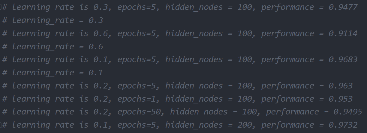
太多的训练实际上会过犹不及,这是由于网络过度拟合训练数据,因此网络在先前没有见到过的新数据上表现不佳。不仅是神经网络,在各种类型的机器学习中,这种过度拟合也是需要注意的。


改变网络形状


测试自己的手写数字

import numpy
# scipy.special for the sigmoid function expit()
import scipy.special
# library for plotting arrays
import matplotlib.pyplot
# ensure the plots are inside this notebook, not an external window
%matplotlib inline
# neural network class definition
# code for a 3-layer neural network, and code for learning the MNIST dataset
class neuralNetwork:
    # initialise the neural network
    def __init__(self, inputnodes, hiddennodes, outputnodes, learningrate):
        # set number of nodes in each input, hidden, output layer
        self.inodes = inputnodes
        self.hnodes = hiddennodes
        self.onodes = outputnodes

        # link weight matrices, wih and who
        # weights inside the arrays are w_i_j, where link is from node i to node j in the next
        # layer
        # w11 w21 w12 w22 etc
        # self.wih = (numpy.random.rand(self.hnodes, self.inodes) - 0.5)
        # self.who = (numpy.random.rand(self.onodes, self.hnodes) - 0.5)
        # 从正态(高斯)分布中抽取随机样本构建权重矩阵
        # numpy.random.normal(mean, std, size)
        # pow(self.hnodes, -0.5)和pow(self.onodes, -0.5)是经验规则
        # 数学家所得到的经验规则是,我们可以在一个节点传入链接数量平方根倒数的大致范围内随机采样,初始化权重。
        self.wih = numpy.random.normal(0.0, pow(self.hnodes, -0.5), (self.hnodes, self.inodes))
        self.who = numpy.random.normal(0.0, pow(self.onodes, -0.5), (self.onodes, self.hnodes))

        # 学习率
        self.lr = learningrate

        # activation function is the sigmoid function
        # 激活函数
        self.activation_function = lambda x: scipy.special.expit(x)
        pass

    # train the neural network
    def train(self, inputs_list, targets_list):
        # convert inputs list to 2d array
        # 把输入值转化为列向量
        inputs = numpy.array(inputs_list, ndmin=2).T
        # 把目标输出值转化为列向量
        targets = numpy.array(targets_list, ndmin=2).T

        # calculate signals into hidden layer
        hidden_inputs = numpy.dot(self.wih, inputs)
        # calculate the signals emerging from hidden layer
        hidden_outputs = self.activation_function(hidden_inputs)

        # calculate signals into output layer
        final_inputs = numpy.dot(self.who, hidden_outputs)
        # calculate the signals emerging from final output layer
        final_outputs = self.activation_function(final_inputs)

        # output layer error is the (target - actual)
        output_errors = targets - final_outputs
        # hidden layer error is the output_errors, split by weights, recombined at hidden nodes
        hidden_errors = numpy.dot(self.who.T, output_errors)

        # update the weights for the links between the hidden and output layers
        # 更新隐藏层到输出层的权重
        self.who += self.lr * numpy.dot((output_errors * final_outputs * (1.0 - final_outputs)), numpy.transpose(hidden_outputs))
        # update the weights for the links between the input and hidden layers
        # 更新输入层到隐藏层的权重
        self.wih += self.lr * numpy.dot((hidden_errors * hidden_outputs * (1.0 - hidden_outputs)), numpy.transpose(inputs))
        pass

    # query the neural network
    def query(self, inputs_list):
        # convert inputs list to 2d array
        # 把输入值转化为列向量
        inputs = numpy.array(inputs_list, ndmin=2).T

        # calculate signals into hidden layer
        hidden_inputs = numpy.dot(self.wih, inputs)
        # calculate the signals emerging from hidden layer
        hidden_outputs = self.activation_function(hidden_inputs)

        # calculate signals into output layer
        final_inputs = numpy.dot(self.who, hidden_outputs)
        # calculate the signals emerging from final output layer
        final_outputs = self.activation_function(final_inputs)
        return final_outputs
# number of input, hidden and output nodes
# input_nodes = 3
# hidden_nodes = 3
# output_nodes = 3
input_nodes = 784
# hidden_nodes = 100
hidden_nodes = 200
# 输出层对应10个label
output_nodes = 10

# learning rate is 0.3, epochs=5, hidden_nodes = 100, performance = 0.9477
# learning_rate = 0.3
# learning rate is 0.6, epochs=5, hidden_nodes = 100, performance = 0.9114
# learning_rate = 0.6
# learning rate is 0.1, epochs=5, hidden_nodes = 100, performance = 0.9683
# learning_rate = 0.1
# learning rate is 0.2, epochs=5, hidden_nodes = 100, performance = 0.963
# learning rate is 0.2, epochs=1, hidden_nodes = 100, performance = 0.953
# learning rate is 0.2, epochs=50, hidden_nodes = 100, performance = 0.9495
# learning rate is 0.1, epochs=5, hidden_nodes = 200, performance = 0.9732
learning_rate = 0.1

# create instance of neural network
n = neuralNetwork(input_nodes, hidden_nodes, output_nodes, learning_rate)

# print(n.query([1.0, 0.5, -1.5]))

# load the mnist training data CSV file into a list
training_data_file = open("mnist_dataset/mnist_train.csv", 'r')
training_data_list = training_data_file.readlines()
training_data_file.close()

# all_values = training_data_list[0].split(',')
# image_array = numpy.asfarray(all_values[1:]).reshape((28, 28))
# matplotlib.pyplot.imshow(image_array, cmap='Greys', interpolation='None')
# matplotlib.pyplot.show()

# scaled_input = (numpy.asfarray(all_values[1:]) / 255.0 * 0.99) + 0.01
# print(scaled_input)

# train the neural network
# 训练网络
# epochs is the number of times the training dataset is used for training
epochs = 5

for e in range(epochs):
    # go through all records in the training data set
    for record in training_data_list:
        # split the record by the ',' commas
        all_values = record.split(',')
        # scale and shift the inputs
        inputs = (numpy.asfarray(all_values[1:]) / 255.0 * 0.99) + 0.01
        # create the target output values (all 0.01 except the desired label which is 0.99)
        targets = numpy.zeros(output_nodes) + 0.01
        # all_values[0] is the target label for this record
        targets[int(all_values[0])] = 0.99
        # 训练网络
        n.train(inputs, targets)
        pass
    pass
from PIL import Image
import numpy as np
from scipy import misc
import matplotlib.pyplot as pyplot

# 将图片输出为二维数组
def loadImage(filename):
    # 读取图片
    im = Image.open(filename)
    # 显示原图
    # im.show()
    # 转换为灰度图
    im = im.convert("L")
    # 以包含像素值的序列对象的形式返回此图像的内容
    img_array = im.getdata()
    # 从一串数据或类似数组的对象中返回一个矩阵
    img_array = np.matrix(img_array)
    # reshape from 28x28 to list of 784 values, invert values
    img_data = 255.0 - img_array.reshape(784)
    # then scale data to range from 0.01 to 1.0
    img_data = (img_data / 255.0 * 0.99) + 0.01
    return img_data

data = loadImage("my_own_images/2828_my_own_3.png")
data.shape
将其从28×28的方块数组变成很长的一串数值,这是我们需要馈送给神经网络的数据。此前,我们已经多次进行这样的操作了。但是,这里比较新鲜的一点是将数组的值减去了255.0。这样做的原因是,常规而言,0指的是黑色,255指的是白色,但是,MNIST数据集使用相反的方式表示,因此不得不将值逆转过来以匹配MNIST数据。

我们需要创建基本的神经网络,这个神经网络使用MNIST训练数据集进行训练,然后,不使用MNIST测试集对网络进行测试,而是使用自己创建的图像数据对网络进行测试
# glob helps select multiple files using patterns
import glob

# our own image test data set
our_own_dataset = []

# load the png image data as test data set
for image_file_name in glob.glob('my_own_images/2828_my_own_?.png'):

    # use the filename to set the correct label
    label = int(image_file_name[-5:-4])

    # load image data from png files into an array
    print ("loading ... ", image_file_name)
    # 将图片输出为二维数组
    img_data = loadImage(image_file_name)

    print(numpy.min(img_data))
    print(numpy.max(img_data))

    # append label and image data to test data set
    record = numpy.append(label, img_data)
    our_own_dataset.append(record)

    pass


# test the neural network withour own images

# load image data from png files into an array
print ("loading ... my_own_images/2828_my_own_image.png")

img_data = loadImage('my_own_images/2828_my_own_image.png')
print("min = ", numpy.min(img_data))
print("max = ", numpy.max(img_data))

# plot image
matplotlib.pyplot.imshow(img_data.reshape(28,28), cmap='Greys', interpolation='None')

# query the network
outputs = n.query(img_data)
print(outputs)

# the index of the highest value corresponds to the label
label = numpy.argmax(outputs)
print("network says ", label)

可以看到,神经网络能够识别我们创建的所有图像,包括有意损坏的数字“3”。只有在识别添加了噪声的数字“6”时失败了。
神经网络黑盒子
神经网络的工作方式是将学习分布到不同的链接权重中。这种方式使得神经网络对损坏具有了弹性,这就像是生物大脑的运行方式。删除一个节点甚至相当多的节点,都不太可能彻底破坏神经网络良好的工作能力。
向后查询


 # backquery the neural network
 # we'll use the same terminology to each item,
 # e.g. targets are the values at the right of the network, albeit used as input
 # e.g. hidden_output is the signal to the right of the middle nodes
 def backquery(self, targets_list):
     # transpose the targets list to a vertical array
     # 把输入值转化为列向量
     final_outputs = numpy.array(targets_list, ndmin=2).T

     # calculate the signal into the final output layer
     # 反函数回到final_inputs的值
     final_inputs = self.inverse_activation_function(final_outputs)

     # calculate the signal out of the hidden layer

     # det = numpy.linalg.det(self.who.T)
     # print("det:", det, '\n')
     # 这里类似于train里面算的ERRORhidden的思想
     hidden_outputs = numpy.dot(self.who.T, final_inputs)
     # scale them back to 0.01 to .99
     hidden_outputs -= numpy.min(hidden_outputs)
     hidden_outputs /= numpy.max(hidden_outputs)
     hidden_outputs *= 0.98
     hidden_outputs += 0.01

     # calculate the signal into the hidden layer
     hidden_inputs = self.inverse_activation_function(hidden_outputs)

     # calculate the signal out of the input layer
     # det2 = numpy.linalg.det(self.wih.T)
     # print("det2:", det2, '\n')
     # 这里类似于train里面算的ERRORhidden的思想
     inputs = numpy.dot(self.wih.T, hidden_inputs)
     # scale them back to 0.01 to .99
     inputs -= numpy.min(inputs)
     inputs /= numpy.max(inputs)
     inputs *= 0.98
     inputs += 0.01

     return inputs
利用现有神经网络反向输出图像
# number of input, hidden and output nodes
# input_nodes = 3
# hidden_nodes = 3
# output_nodes = 3
input_nodes = 784
# hidden_nodes = 100
hidden_nodes = 200
# 输出层对应10个label
output_nodes = 10

# learning rate is 0.3, epochs=5, hidden_nodes = 100, performance = 0.9477
# learning_rate = 0.3
# learning rate is 0.6, epochs=5, hidden_nodes = 100, performance = 0.9114
# learning_rate = 0.6
# learning rate is 0.1, epochs=5, hidden_nodes = 100, performance = 0.9683
# learning_rate = 0.1
# learning rate is 0.2, epochs=5, hidden_nodes = 100, performance = 0.963
# learning rate is 0.2, epochs=1, hidden_nodes = 100, performance = 0.953
# learning rate is 0.2, epochs=50, hidden_nodes = 100, performance = 0.9495
# learning rate is 0.1, epochs=5, hidden_nodes = 200, performance = 0.9732
learning_rate = 0.1

# create instance of neural network
n = neuralNetwork(input_nodes, hidden_nodes, output_nodes, learning_rate)

# print(n.query([1.0, 0.5, -1.5]))

# load the mnist training data CSV file into a list
training_data_file = open("mnist_dataset/mnist_train.csv", 'r')
training_data_list = training_data_file.readlines()
training_data_file.close()

# all_values = training_data_list[0].split(',')
# image_array = numpy.asfarray(all_values[1:]).reshape((28, 28))
# matplotlib.pyplot.imshow(image_array, cmap='Greys', interpolation='None')
# matplotlib.pyplot.show()

# scaled_input = (numpy.asfarray(all_values[1:]) / 255.0 * 0.99) + 0.01
# print(scaled_input)

# train the neural network
# 训练网络
# epochs is the number of times the training dataset is used for training
epochs = 5

for e in range(epochs):
    # go through all records in the training data set
    for record in training_data_list:
        # split the record by the ',' commas
        all_values = record.split(',')
        # scale and shift the inputs
        inputs = (numpy.asfarray(all_values[1:]) / 255.0 * 0.99) + 0.01
        # create the target output values (all 0.01 except the desired label which is 0.99)
        targets = numpy.zeros(output_nodes) + 0.01
        # all_values[0] is the target label for this record
        targets[int(all_values[0])] = 0.99
        # 训练网络
        n.train(inputs, targets)
        pass
    pass


# load the mnist test data CSV file into a list
test_data_file = open("mnist_dataset/mnist_test.csv", 'r')
test_data_list = test_data_file.readlines()
test_data_file.close()

# test the neural network
# 测试网络,记分卡
# scorecard for how well the network performs, initially empty
scorecard = []

# go through all the records in the test dataset
for record in test_data_list:
    # split the record by the ',' commas
    all_values = record.split(',')
    # correct answer is first value
    correct_label = int(all_values[0])
    # print(correct_label, "correct label")
    # scale and shift the inputs
    # 调整输入层输入数据
    inputs = (numpy.asfarray(all_values[1:]) / 255.0 * 0.99) + 0.01
    # query the network
    # 查询网络
    outputs = n.query(inputs)
    # the index of the highest value corresponds to the label
    label = numpy.argmax(outputs)
    # print(label, "network's answer")
    # append correct or incorrect to list
    if(label == correct_label):
        # network's answer matches correct answer, and 1 to scorecard
        scorecard.append(1)
    else:
        # network's answer doesn't match correct answer, add 0 to scorecard
        scorecard.append(0)
        pass
    pass

# calculate the performance score, the fraction of correct answers
scorecard_array = numpy.asarray(scorecard)
print("performance =", scorecard_array.sum() / scorecard_array.size)

# run the network backwards, given a label, see what imgae it produces

# label to test
label = 0
# create the output signals for this label
targets = numpy.zeros(output_nodes) + 0.01
targets[label] = 0.99
# print(targets)

# get image data
image_data = n.backquery(targets)

# plot image data
matplotlib.pyplot.imshow(image_data.reshape(28, 28), cmap='Greys', interpolation='None')


创建新的训练数据:旋转图像
如果思考一下MNIST训练数据,你就会意识到,这是关于人们所书写数字的一个相当丰富的样本集。这里有各种各样、各种风格的书写,有的写得很好,有的写得很糟。
神经网络必须尽可能多地学习这些变化类型。在这里,有多种形式的数字“4”,有些被压扁了,有些比较宽,有些进行了旋转,有些顶部是开放的,有些顶部是闭合的,这对神经网络的学习都是有帮助的。
一个很酷的想法就是利用已有的样本,通过顺时针或逆时针旋转它们,比如说旋转10度,创建新的样本。对于每一个训练样本而言,我们能够生成两个额外的样本。我们可以使用不同的旋转角度创建更多的样本,但是,目前,让我们只尝试+10和-10两个角度,看看这种想法能不能成功。
由于我们将神经网络设计成为接收一长串输入信号,因此输入的是784长的一串一维数字。我们需要将这一长串数字重新变成28×28的数组,这样就可以旋转这个数组,然后在将这个数组馈送到神经网络之前,将数组解开,重新变成一长串的784个信号。
# create rotated variations
# rotated anticlockwise by 10 degrees
inputs_plus10_img = scipy.ndimage.rotate(scaled_input, 10.0, cval=0.01, order=1, reshape=False)
# rotated clockwise by 10 degrees
inputs_minus10_img = scipy.ndimage.rotate(scaled_input, -10.0, cval=0.01, order=1, reshape=False)
可以看到,原先的scaled_input数组被重新转变为28x28的数组,然后进行了调整。reshape=False,这个参数防止程序库过分“热心”,将图像压扁,使得数组旋转后可以完全适合,而没有剪掉任何部分。在原始图像中,一些数组元素不存在,但是现在这些数组元素进入了视野,cval就是用来填充数组元素的值。由于我们要移动输入值范围,避免0作为神经网络的输入值,因此不使用0.0作为默认值,而是使用0.01作为默认值。
scipy.ndimage.rotate
官方文档

旋转数据集“1”
小型MNIST训练集的记录6(第7条记录)是一个手写数字“1”。在下图中可以看到,原先的数字图片和使用代码生成的两个额外的变化形式。


添加旋转图像数据集进行神经网络的训练和测试
# numpy provides arrays and useful functions for working with them
import numpy
# scipy.special for the sigmoid function expit()
import scipy.special
# scipy.ndimage for rotating image arrays
import scipy.ndimage

# neural network class definition
# code for a 3-layer neural network, and code for learning the MNIST dataset
class neuralNetwork:
    # initialise the neural network
    def __init__(self, inputnodes, hiddennodes, outputnodes, learningrate):
        # set number of nodes in each input, hidden, output layer
        self.inodes = inputnodes
        self.hnodes = hiddennodes
        self.onodes = outputnodes

        # link weight matrices, wih and who
        # weights inside the arrays are w_i_j, where link is from node i to node j in the next
        # layer
        # w11 w21 w12 w22 etc
        # self.wih = (numpy.random.rand(self.hnodes, self.inodes) - 0.5)
        # self.who = (numpy.random.rand(self.onodes, self.hnodes) - 0.5)
        # 从正态(高斯)分布中抽取随机样本构建权重矩阵
        # numpy.random.normal(mean, std, size)
        # pow(self.hnodes, -0.5)和pow(self.onodes, -0.5)是经验规则
        # 数学家所得到的经验规则是,我们可以在一个节点传入链接数量平方根倒数的大致范围内随机采样,初始化权重。
        self.wih = numpy.random.normal(0.0, pow(self.hnodes, -0.5), (self.hnodes, self.inodes))
        self.who = numpy.random.normal(0.0, pow(self.onodes, -0.5), (self.onodes, self.hnodes))

        # 学习率
        self.lr = learningrate

        # activation function is the sigmoid function
        # 激活函数
        self.activation_function = lambda x: scipy.special.expit(x)
        self.inverse_activation_function = lambda x: scipy.special.logit(x)
        pass

    # train the neural network
    def train(self, inputs_list, targets_list):
        # convert inputs list to 2d array
        # 把输入值转化为列向量
        inputs = numpy.array(inputs_list, ndmin=2).T
        # 把目标输出值转化为列向量
        targets = numpy.array(targets_list, ndmin=2).T

        # calculate signals into hidden layer
        hidden_inputs = numpy.dot(self.wih, inputs)
        # calculate the signals emerging from hidden layer
        hidden_outputs = self.activation_function(hidden_inputs)

        # calculate signals into output layer
        final_inputs = numpy.dot(self.who, hidden_outputs)
        # calculate the signals emerging from final output layer
        final_outputs = self.activation_function(final_inputs)

        # output layer error is the (target - actual)
        output_errors = targets - final_outputs
        # hidden layer error is the output_errors, split by weights, recombined at hidden nodes
        hidden_errors = numpy.dot(self.who.T, output_errors)

        # update the weights for the links between the hidden and output layers
        # 更新隐藏层到输出层的权重
        self.who += self.lr * numpy.dot((output_errors * final_outputs * (1.0 - final_outputs)), numpy.transpose(hidden_outputs))
        # update the weights for the links between the input and hidden layers
        # 更新输入层到隐藏层的权重
        self.wih += self.lr * numpy.dot((hidden_errors * hidden_outputs * (1.0 - hidden_outputs)), numpy.transpose(inputs))
        pass

    # query the neural network
    def query(self, inputs_list):
        # convert inputs list to 2d array
        # 把输入值转化为列向量
        inputs = numpy.array(inputs_list, ndmin=2).T

        # calculate signals into hidden layer
        hidden_inputs = numpy.dot(self.wih, inputs)
        # calculate the signals emerging from hidden layer
        hidden_outputs = self.activation_function(hidden_inputs)

        # calculate signals into output layer
        final_inputs = numpy.dot(self.who, hidden_outputs)
        # calculate the signals emerging from final output layer
        final_outputs = self.activation_function(final_inputs)
        return final_outputs

    # backquery the neural network
    # we'll use the same terminology to each item,
    # e.g. targets are the values at the right of the network, albeit used as input
    # e.g. hidden_output is the signal to the right of the middle nodes
    def backquery(self, targets_list):
        # transpose the targets list to a vertical array
        # 把输入值转化为列向量
        final_outputs = numpy.array(targets_list, ndmin=2).T

        # calculate the signal into the final output layer
        # 反函数回到final_inputs的值
        final_inputs = self.inverse_activation_function(final_outputs)

        # calculate the signal out of the hidden layer

        # det = numpy.linalg.det(self.who.T)
        # print("det:", det, '\n')
        # 这里类似于train里面算的ERRORhidden的思想
        hidden_outputs = numpy.dot(self.who.T, final_inputs)
        # scale them back to 0.01 to .99
        hidden_outputs -= numpy.min(hidden_outputs)
        hidden_outputs /= numpy.max(hidden_outputs)
        hidden_outputs *= 0.98
        hidden_outputs += 0.01

        # calculate the signal into the hidden layer
        hidden_inputs = self.inverse_activation_function(hidden_outputs)

        # calculate the signal out of the input layer
        # det2 = numpy.linalg.det(self.wih.T)
        # print("det2:", det2, '\n')
        # 这里类似于train里面算的ERRORhidden的思想
        inputs = numpy.dot(self.wih.T, hidden_inputs)
        # scale them back to 0.01 to .99
        inputs -= numpy.min(inputs)
        inputs /= numpy.max(inputs)
        inputs *= 0.98
        inputs += 0.01

        return inputs

# number of input, hidden and output nodes
# input_nodes = 3
# hidden_nodes = 3
# output_nodes = 3
input_nodes = 784
# hidden_nodes = 100
hidden_nodes = 200
# 输出层对应10个label
output_nodes = 10

# learning rate is 0.3, epochs=5, hidden_nodes = 100, performance = 0.9477
# learning_rate = 0.3
# learning rate is 0.6, epochs=5, hidden_nodes = 100, performance = 0.9114
# learning_rate = 0.6
# learning rate is 0.1, epochs=5, hidden_nodes = 100, performance = 0.9683
# learning_rate = 0.1
# learning rate is 0.2, epochs=5, hidden_nodes = 100, performance = 0.963
# learning rate is 0.2, epochs=1, hidden_nodes = 100, performance = 0.953
# learning rate is 0.2, epochs=50, hidden_nodes = 100, performance = 0.9495
# learning rate is 0.1, epochs=5, hidden_nodes = 200, performance = 0.9732
learning_rate = 0.01

# create instance of neural network
n = neuralNetwork(input_nodes, hidden_nodes, output_nodes, learning_rate)

# print(n.query([1.0, 0.5, -1.5]))

# load the mnist training data CSV file into a list
training_data_file = open("mnist_dataset/mnist_train.csv", 'r')
training_data_list = training_data_file.readlines()
training_data_file.close()

# all_values = training_data_list[0].split(',')
# image_array = numpy.asfarray(all_values[1:]).reshape((28, 28))
# matplotlib.pyplot.imshow(image_array, cmap='Greys', interpolation='None')
# matplotlib.pyplot.show()

# scaled_input = (numpy.asfarray(all_values[1:]) / 255.0 * 0.99) + 0.01
# print(scaled_input)

# train the neural network
# 训练网络
# epochs is the number of times the training dataset is used for training
epochs = 10

for e in range(epochs):
    # go through all records in the training data set
    for record in training_data_list:
        # split the record by the ',' commas
        all_values = record.split(',')
        # scale and shift the inputs
        inputs = (numpy.asfarray(all_values[1:]) / 255.0 * 0.99) + 0.01
        # create the target output values (all 0.01 except the desired label which is 0.99)
        targets = numpy.zeros(output_nodes) + 0.01
        # all_values[0] is the target label for this record
        targets[int(all_values[0])] = 0.99
        # 训练网络
        n.train(inputs, targets)

        ## create rotated variations
        # rotated anticlockwise by x degrees
        inputs_plusx_img = scipy.ndimage.rotate(inputs.reshape(28, 28), 10, cval=0.01, reshape=False)
        n.train(inputs_plusx_img.reshape(784), targets)
        # rotated clockwise by x degrees
        inputs_minusx_img = scipy.ndimage.rotate(inputs.reshape(28, 28), -10, cval=0.01, reshape=False)
        n.train(inputs_minusx_img.reshape(784), targets)

        pass
    pass


# load the mnist test data CSV file into a list
test_data_file = open("mnist_dataset/mnist_test.csv", 'r')
test_data_list = test_data_file.readlines()
test_data_file.close()

# test the neural network
# 测试网络,记分卡
# scorecard for how well the network performs, initially empty
scorecard = []

# go through all the records in the test dataset
for record in test_data_list:
    # split the record by the ',' commas
    all_values = record.split(',')
    # correct answer is first value
    correct_label = int(all_values[0])
    # print(correct_label, "correct label")
    # scale and shift the inputs
    # 调整输入层输入数据
    inputs = (numpy.asfarray(all_values[1:]) / 255.0 * 0.99) + 0.01
    # query the network
    # 查询网络
    outputs = n.query(inputs)
    # the index of the highest value corresponds to the label
    label = numpy.argmax(outputs)
    # print(label, "network's answer")
    # append correct or incorrect to list
    if(label == correct_label):
        # network's answer matches correct answer, and 1 to scorecard
        scorecard.append(1)
    else:
        # network's answer doesn't match correct answer, add 0 to scorecard
        scorecard.append(0)
        pass
    pass

# calculate the performance score, the fraction of correct answers
scorecard_array = numpy.asarray(scorecard)
print("performance =", scorecard_array.sum() / scorecard_array.size)