在线的latex编辑和编译工具:overleaf
论文最终展现出来的就是一个PDF格式的文档。
当然可以使用word,但光排版这件事情,就能耗费你一半的精力。
正确的答案是,使用latex,它是一个专业的排版工具,按照latex的语法进行写作,执行编译就能够得到PDF文件。它的语法包含了如何排版,虽然相比word上手要慢,但在排版这件事情上,入门级别的latex语法,你要达到精通word的水平。
latex如何使用呢?当然,要安装编译器,再安装编辑器,本地一通配置,偶尔会遇到些问题,凭着强大的谷歌搜索,倒也不是什么难事。配置本地环境,不如直接使用在线编辑器。
http://www.overleaf.com
- 注册即用,免去本地latex环境安装的痛苦。
- 多人合作,共同编辑。
- 富文本编辑模式,比写latex源码舒服些。
- 随时可以完成在线编译,查看PDF。
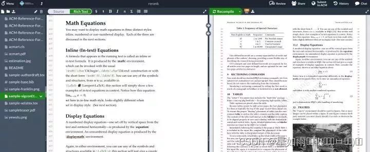
按照overleaf的开始流程,有选择模板的过程,模板怎么选,还是要看投稿的期刊或者会议的要求。以KDD为例,在它的KDD 2019 Call for Research Papers页面上,给出了模板格式,看看能不能在overleaf上找到。
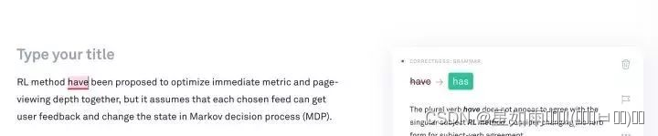
grammarly:语法纠错神器
https://app.grammarly.com/
在这编辑文章的一句或一段话,语法出错了会有提示,低级的语法错误都能够避免。
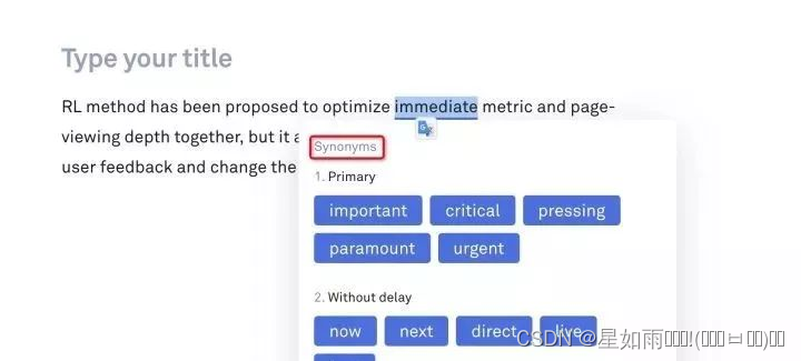
除了语法纠错之外,还有同意替换功能,我的塑料英语能想到的词汇都太过常见,不够精准(逼格不足),选中词就可以同义替换了。
建议在word软件中安装grammarly插件,直接可用在word中进行语法校对和纠正。
论文绘图工具
本人在写机器学习相关论文的时候,很多图片是用matplotlib和seaborn画的,但是,我还有一个神器,Scikit-plot,通过这个神器,画出了更加高大上的机器学习图,本文对Scikit-plot做下简单介绍。
安装说明
安装Scikit-plot非常简单,直接用命令: pip install scikit-plot
即可完成安装。
仓库地址:https://github.com/reiinakano/scikit-plot
里面有使用说明和样例(py和ipynb格式)。
使用说明
简单举几个例子:
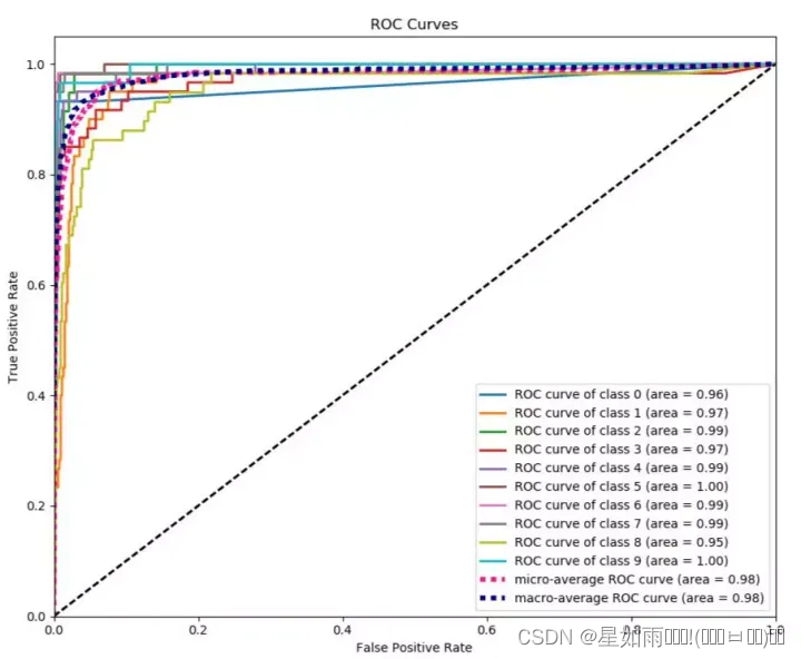
比如画出分类评级指标的ROC曲线的完整代码:
from sklearn.datasets import load_digits
from sklearn.model_selection import train_test_split
from sklearn.naive_bayes import GaussianNB
X, y = load_digits(return_X_y=True)
X_train, X_test, y_train, y_test = train_test_split(X, y, test_size=0.33)
nb = GaussianNB()
nb.fit(X_train, y_train)
predicted_probas = nb.predict_proba(X_test)
# The magic happens here
import matplotlib.pyplot as plt
import scikitplot as skplt
skplt.metrics.plot_roc(y_test, predicted_probas)
plt.show()
效果如图(相当高大上!)
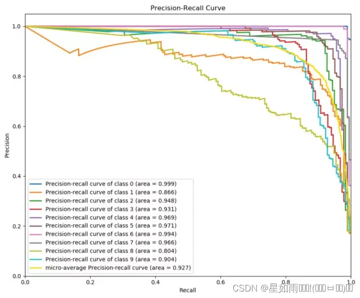
P-R曲线就是精确率precision vs 召回率recall 曲线,以recall作为横坐标轴,precision作为纵坐标轴。首先解释一下精确率和召回率。
import matplotlib.pyplot as plt
from sklearn.naive_bayes import GaussianNB
from sklearn.datasets import load_digits as load_data
import scikitplot as skplt
# Load dataset
X, y = load_data(return_X_y=True)
# Create classifier instance then fit
nb = GaussianNB()
nb.fit(X,y)
# Get predicted probabilities
y_probas = nb.predict_proba(X)
skplt.metrics.plot_precision_recall_curve(y, y_probas, cmap='nipy_spectral')
plt.show()
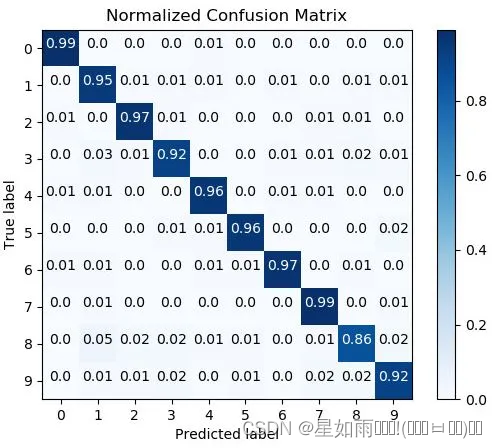
混淆矩阵是分类的重要评价标准,下面代码是用随机森林对鸢尾花数据集进行分类,分类结果画一个归一化的混淆矩阵。
from sklearn.ensemble import RandomForestClassifier
from sklearn.datasets import load_digits as load_data
from sklearn.model_selection import cross_val_predict
import matplotlib.pyplot as plt
import scikitplot as skplt
X, y = load_data(return_X_y=True)
# Create an instance of the RandomForestClassifier
classifier = RandomForestClassifier()
# Perform predictions
predictions = cross_val_predict(classifier, X, y)
plot = skplt.metrics.plot_confusion_matrix(y, predictions, normalize=True)
plt.show()
其他图如学习曲线、特征重要性、聚类的肘点等等,都可以用几行代码搞定。
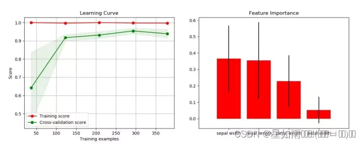
本章对Scikit-plot做下简单介绍,这是一个机器学习的画图神器,几行代码就能画出高大上的机器学习图。