
作者 | Lavanya Shukla
译者 | Monanfei
责编 | 夕颜
出品 | AI科技大本营(id:rgznai100)
导读:刚开始接触数据竞赛时,我们可能会被一些高大上的技术吓到。各界大佬云集,各种技术令人眼花缭乱,新手们就像蜉蝣一般渺小无助。今天本文就分享一下在 kaggle 的竞赛中,参赛者取得 top0.3% 的经验和技巧。让我们开始吧!
Top 0.3% 模型概览
赛题和目标
数据集中的每一行都描述了某一匹马的特征
在已知这些特征的条件下,预测每匹马的销售价格
预测价格对数和真实价格对数的RMSE(均方根误差)作为模型的评估指标。将RMSE转化为对数尺度,能够保证廉价马匹和高价马匹的预测误差,对模型分数的影响较为一致。
模型训练过程中的重要细节
交叉验证:使用12-折交叉验证
模型:在每次交叉验证中,同时训练七个模型(ridge, svr, gradient boosting, random forest, xgboost, lightgbm regressors)
Stacking 方法:使用 xgboot 训练了元 StackingCVRegressor 学习器
模型融合:所有训练的模型都会在不同程度上过拟合,因此,为了做出最终的预测,将这些模型进行了融合,得到了鲁棒性更强的预测结果
模型性能
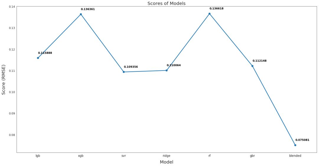
从下图可以看出,融合后的模型性能最好,RMSE 仅为 0.075,该融合模型用于最终预测。
In[1]:
from IPython.display import Image
Image("../input/kernel-files/model_training_advanced_regression.png")
Output[1]:
现在让我们正式开始吧!
In[2]:
# Essentials
import numpy as np
import pandas as pd
import datetime
import random
# Plots
import seaborn as sns
import matplotlib.pyplot as plt # Models
from sklearn.ensemble import RandomForestRegressor, GradientBoostingRegressor, AdaBoostRegressor, BaggingRegressor
from sklearn.kernel_ridge import KernelRidge
from sklearn.linear_model import Ridge, RidgeCV
from sklearn.linear_model import ElasticNet, ElasticNetCV
from sklearn.svm import SVR
from mlxtend.regressor import StackingCVRegressor
import lightgbm as lgb
from lightgbm import LGBMRegressor
from xgboost import XGBRegressor # Stats
from scipy.stats import skew, norm
from scipy.special import boxcox1p
from scipy.stats import boxcox_normmax # Misc
from sklearn.model_selection import GridSearchCV
from sklearn.model_selection import KFold, cross_val_score
from sklearn.metrics import mean_squared_error
from sklearn.preprocessing import OneHotEncoder
from sklearn.preprocessing import LabelEncoder
from sklearn.pipeline import make_pipeline
from sklearn.preprocessing import scale
from sklearn.preprocessing import StandardScaler
from sklearn.preprocessing import RobustScaler
from sklearn.decomposition import PCA pd.set_option('display.max_columns', None) # Ignore useless warnings
import warnings
warnings.filterwarnings(action="ignore")
pd.options.display.max_seq_items = 8000
pd.options.display.max_rows = 8000 import os
print(os.listdir("../input/kernel-fi
Output[2]:
['model_training_advanced_regression.png']
In[3]:
# Read in the dataset as a dataframe
train = pd.read_csv('../input/house-prices-advanced-regression-techniques/train.csv')
test = pd.read_csv('../input/house-prices-advanced-regression-techniques/test.csv')
train.shape, test.shape
Output[3]:
((1460, 81), (1459, 80))
EDA
目标
数据集中的每一行都描述了某一匹马的特征
在已知这些特征的条件下,预测每匹马的销售价格
对原始数据进行可视化
In[4]:
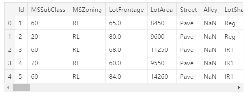
# Preview the data we're working with
train.head()
Output[5]:
SalePrice:目标值的特性探究
In[5]:
sns.set_style("white")
sns.set_color_codes(palette='deep')
f, ax = plt.subplots(figsize=(8, 7))
#Check the new distribution
sns.distplot(train['SalePrice'], color="b");
ax.xaxis.grid(False)
ax.set(ylabel="Frequency")
ax.set(xlabel="SalePrice")
ax.set(title="SalePrice distribution")
sns.despine(trim=True, left=True)
plt.show() 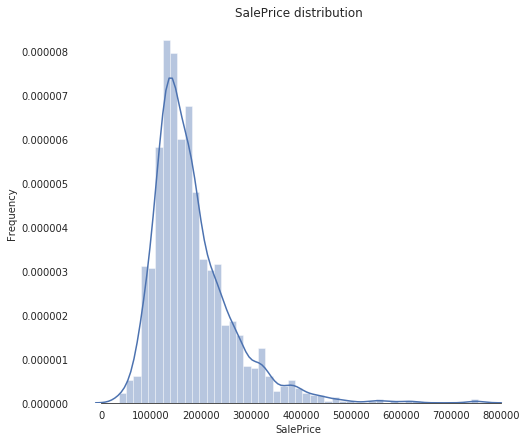
In[6]:
# Skew and kurt
print("Skewness: %f" % train['SalePrice'].skew())
print("Kurtosis: %f" % train['SalePrice'].kurt())
Skewness: 1.882876
Kurtosis: 6.536282
可用的特征:深入探索
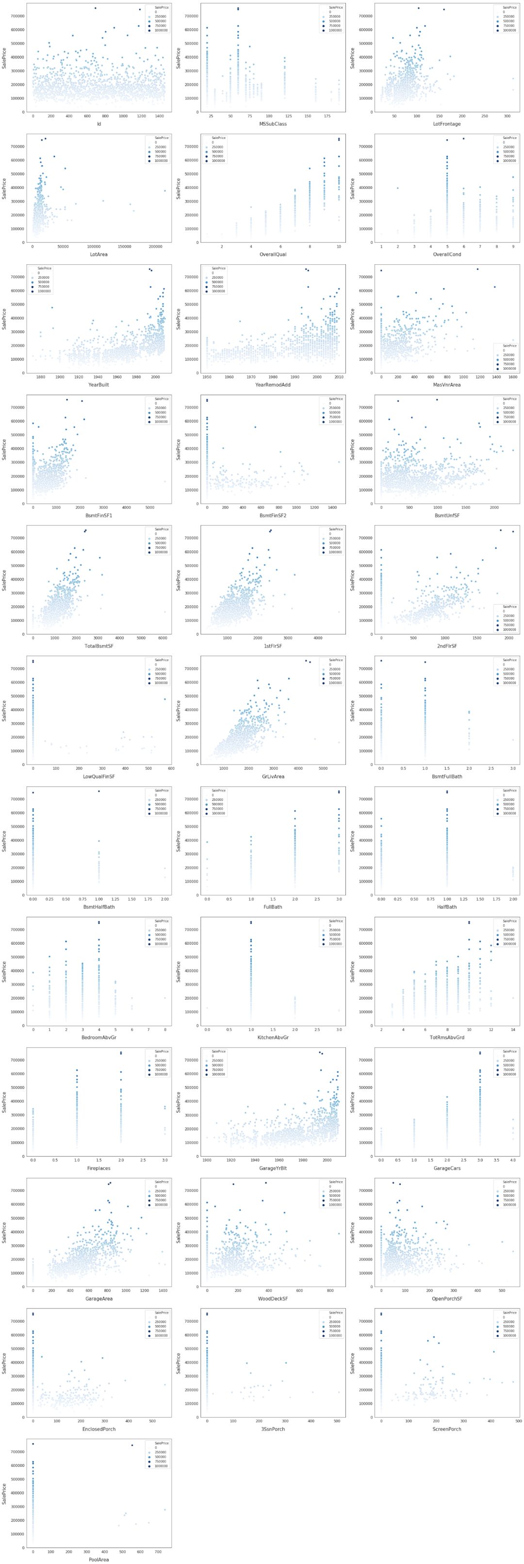
数据可视化
In[7]:
# Finding numeric features
numeric_dtypes = ['int16', 'int32', 'int64', 'float16', 'float32', 'float64']
numeric = []
for i in train.columns:	if train[i].dtype in numeric_dtypes:	if i in ['TotalSF', 'Total_Bathrooms','Total_porch_sf','haspool','hasgarage','hasbsmt','hasfireplace']:	pass	else:	numeric.append(i)
# visualising some more outliers in the data values
fig, axs = plt.subplots(ncols=2, nrows=0, figsize=(12, 120))
plt.subplots_adjust(right=2)
plt.subplots_adjust(top=2)
sns.color_palette("husl", 8)
for i, feature in enumerate(list(train[numeric]), 1):	if(feature=='MiscVal'):	break	plt.subplot(len(list(numeric)), 3, i)	sns.scatterplot(x=feature, y='SalePrice', hue='SalePrice', palette='Blues', data=train)	plt.xlabel('{}'.format(feature), size=15,labelpad=12.5)	plt.ylabel('SalePrice', size=15, labelpad=12.5)	for j in range(2):	plt.tick_params(axis='x', labelsize=12)	plt.tick_params(axis='y', labelsize=12)	plt.legend(loc='best', prop={'size': 10})	plt.show()
探索这些特征以及 SalePrice 的相关性
In[8]:
corr = train.corr()
plt.subplots(figsize=(15,12))
sns.heatmap(corr, vmax=0.9, cmap="Blues", square=True)
Output[8]:
<matplotlib.axes._subplots.AxesSubplot at 0x7ff0e416e4e0>
选取部分特征,可视化它们和 SalePrice 的相关性
Input[9]:
data = pd.concat([train['SalePrice'], train['OverallQual']], axis=1)
f, ax = plt.subplots(figsize=(8, 6))
fig = sns.boxplot(x=train['OverallQual'], y="SalePrice", data=data)
fig.axis(ymin=0, ymax=800000); 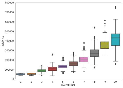
Input[10]:
data = pd.concat([train['SalePrice'], train['YearBuilt']], axis=1)
f, ax = plt.subplots(figsize=(16, 8))
fig = sns.boxplot(x=train['YearBuilt'], y="SalePrice", data=data)
fig.axis(ymin=0, ymax=800000);
plt.xticks(rotation=45); 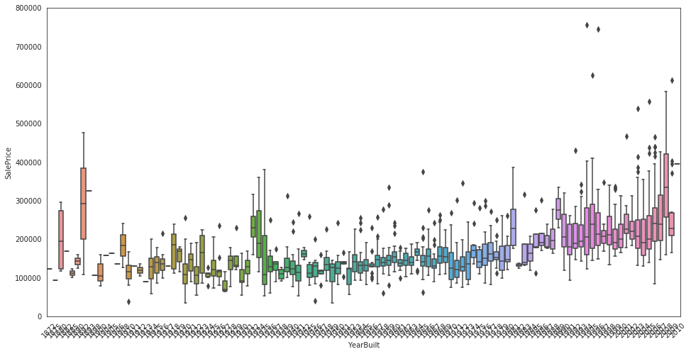
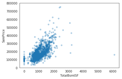
Input[11]:
data = pd.concat([train['SalePrice'], train['TotalBsmtSF']], axis=1)
data.plot.scatter(x='TotalBsmtSF', y='SalePrice', alpha=0
.3, ylim=(0,800000));
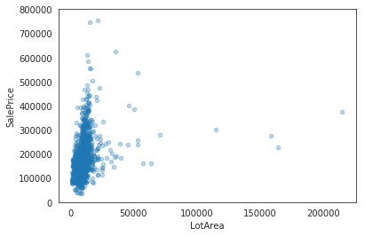
Input[12]:
data = pd.concat([train['SalePrice'], train['LotArea']], axis=1)
data.plot.scatter(x='LotArea', y='SalePrice', alpha=0.3, y
lim=(0,800000));
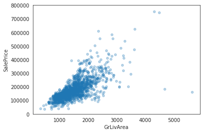
Input[13]:
data = pd.concat([train['SalePrice'], train['GrLivArea']], axis=1)
data.plot.scatter(x='GrLivArea', y='SalePrice', alpha=0.3,
ylim=(0,800000));
Input[14]:
# Remove the Ids from train and test, as they are unique for each row and hence not useful for the model
train_ID = train['Id']
test_ID = test['Id']
train.drop(['Id'], axis=1, inplace=True)
test.drop(['Id'], axis=1, inplace=True)
train.shape, test.shape
Output[14]:
((1460, 80), (1459, 79))
可视化 salePrice 的分布
Input[15]:
sns.set_style("white")
sns.set_color_codes(palette='deep')
f, ax = plt.subplots(figsize=(8, 7))
#Check the new distribution
sns.distplot(train['SalePrice'], color="b");
ax.xaxis.grid(False)
ax.set(ylabel="Frequency")
ax.set(xlabel="SalePrice")
ax.set(title="SalePrice distribution")
sns.despine(trim=True, left=True)
plt.show()
从上图中可以看出,SalePrice 有点向右边倾斜,由于大多数机器学习模型对非正态分布的数据的效果不佳,因此,我们对数据进行变换,修正这种倾斜:log(1+x)
Input[16]:
# log(1+x) transform
train["SalePrice"] = np.log1p(train["SalePrice"])
对 SalePrice 重新进行可视化
Input[17]:
sns.set_style("white")
sns.set_color_codes(palette='deep')
f, ax = plt.subplots(figsize=(8, 7))
#Check the new distribution
sns.distplot(train['SalePrice'] , fit=norm, color="b");	# Get the fitted parameters used by the function
(mu, sigma) = norm.fit(train['SalePrice'])
print( '\n mu = {:.2f} and sigma = {:.2f}\n'.format(mu, sigma))	#Now plot the distribution
plt.legend(['Normal dist. ($\mu=$ {:.2f} and $\sigma=$ {:.2f} )'.format(mu, sigma)],	loc='best')
ax.xaxis.grid(False)
ax.set(ylabel="Frequency")
ax.set(xlabel="SalePrice")
ax.set(title="SalePrice distribution")
sns.despine(trim=True, left=True)	plt.show
mu = 12.02 and sigma = 0.40
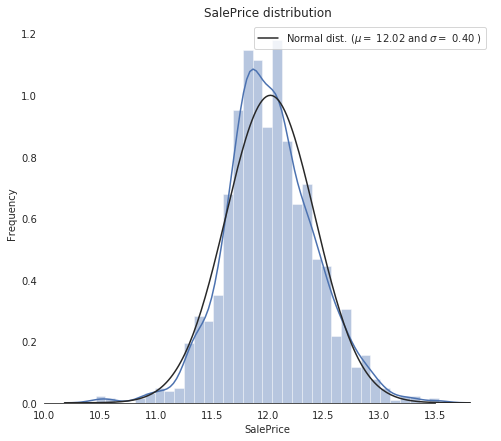
从图中可以看到,当前的 SalePrice 已经变成了正态分布
Input[18]:
# Remove outliers
train.drop(train[(train['OverallQual']<5) & (train['SalePrice']>200000)].index, inplace=True)
train.drop(train[(train['GrLivArea']>4500) & (train['SalePrice']<300000)].index, inplace=True)
train.reset_index(drop=True, inplace=True)
Input[19]:
# Split features and labels
train_labels = train['SalePrice'].reset_index(drop=True)
train_features = train.drop(['SalePrice'], axis=1)
test_features = test
# Combine train and test features in order to apply the feature transformation pipeline to the entire dataset
all_features = pd.concat([train_features, test_features]).reset_index(drop=True)
all_features.shape
Input[19]:
(2917, 79)
填充缺失值
Input[20]:
# determine the threshold for missing values
def percent_missing(df):	data = pd.DataFrame(df)	df_cols = list(pd.DataFrame(data))	dict_x = {}	for i in range(0, len(df_cols)):	dict_x.update({df_cols[i]: round(data[df_cols[i]].isnull().mean()*100,2)})	return dict_x	missing = percent_missing(all_features)
df_miss = sorted(missing.items(), key=lambda x: x[1], reverse=True)
print('Percent of missing data')
df_miss[0:10]
Percent of missing data
Output[20]:
[('PoolQC', 99.69),
('MiscFeature', 96.4),
('Alley', 93.21),
('Fence', 80.43),
('FireplaceQu', 48.68),
('LotFrontage', 16.66),
('GarageYrBlt', 5.45),
('GarageFinish', 5.45),
('GarageQual', 5.45),
('GarageCond', 5.45)]
Input[21]:
# Visualize missing values
sns.set_style("white")
f, ax = plt.subplots(figsize=(8, 7))
sns.set_color_codes(palette='deep')
missing = round(train.isnull().mean()*100,2)
missing = missing[missing > 0]
missing.sort_values(inplace=True)
missing.plot.bar(color="b")
# Tweak the visual presentation
ax.xaxis.grid(False)
ax.set(ylabel="Percent of missing values")
ax.set(xlabel="Features")
ax.set(title="Percent missing data by feature")
sns.despine(trim=True, left=True) 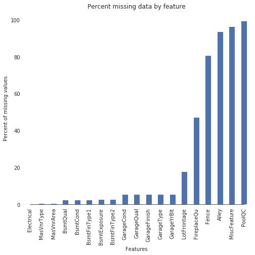
接下来,我们将分别对每一列填充缺失值
Input[22]:
# Some of the non-numeric predictors are stored as numbers; convert them into strings
all_features['MSSubClass'] = all_features['MSSubClass'].apply(str)
all_features['YrSold'] = all_features['YrSold'].astype(str)
all_features['MoSold'] = all_features['MoSold'].astype(str)
Input[23]:
def handle_missing(features): # the data description states that NA refers to typical ('Typ') values features['Functional'] = features['Functional'].fillna('Typ') # Replace the missing values in each of the columns below with their mode features['Electrical'] = features['Electrical'].fillna("SBrkr") features['KitchenQual'] = features['KitchenQual'].fillna("TA") features['Exterior1st'] = features['Exterior1st'].fillna(features['Exterior1st'].mode()[0]) features['Exterior2nd'] = features['Exterior2nd'].fillna(features['Exterior2nd'].mode()[0]) features['SaleType'] = features['SaleType'].fillna(features['SaleType'].mode()[0]) features['MSZoning'] = features.groupby('MSSubClass')['MSZoning'].transform(lambda x: x.fillna(x.mode()[0])) # the data description stats that NA refers to "No Pool" features["PoolQC"] = features["PoolQC"].fillna("None") # Replacing the missing values with 0, since no garage = no cars in garage for col in ('GarageYrBlt', 'GarageArea', 'GarageCars'): features[col] = features[col].fillna(0) # Replacing the missing values with None for col in ['GarageType', 'GarageFinish', 'GarageQual', 'GarageCond']: features[col] = features[col].fillna('None') # NaN values for these categorical basement features, means there's no basement for col in ('BsmtQual', 'BsmtCond', 'BsmtExposure', 'BsmtFinType1', 'BsmtFinType2'): features[col] = features[col].fillna('None') # Group the by neighborhoods, and fill in missing value by the median LotFrontage of the neighborhood features['LotFrontage'] = features.groupby('Neighborhood')['LotFrontage'].transform(lambda x: x.fillna(x.median())) # We have no particular intuition around how to fill in the rest of the categorical features # So we replace their missing values with None objects = [] for i in features.columns: if features[i].dtype == object: objects.append(i) features.update(features[objects].fillna('None')) # And we do the same thing for numerical features, but this time with 0s numeric_dtypes = ['int16', 'int32', 'int64', 'float16', 'float32', 'float64'] numeric = [] for i in features.columns: if features[i].dtype in numeric_dtypes: numeric.append(i) features.update(features[numeric].fillna(0)) return features all_features = handle_missing(all_featuresInput[24]:
# Let's make sure we handled all the missing values
missing = percent_missing(all_features)
df_miss = sorted(missing.items(), key=lambda x: x[1], reverse=True)
print('Percent of missing data')
df_miss[0:10]
Output[14]:
Percent of missing data
[('MSSubClass', 0.0),
('MSZoning', 0.0),
('LotFrontage', 0.0),
('LotArea', 0.0),
('Street', 0.0),
('Alley', 0.0),
('LotShape', 0.0),
('LandContour', 0.0),
('Utilities', 0.0),
('LotConfig', 0.0)]
从上面的结果可以看到,所有缺失值已经填充完毕
调整分布倾斜的特征
Input[25]:
# Fetch all numeric features
numeric_dtypes = ['int16', 'int32', 'int64', 'float16', 'float32', 'float64']
numeric = []
for i in all_features.columns:	if all_features[i].dtype in numeric_dtypes:	numeric.append(i)
Input[26]:
# Create box plots for all numeric features
sns.set_style("white")
f, ax = plt.subplots(figsize=(8, 7))
ax.set_xscale("log")
ax = sns.boxplot(data=all_features[numeric] , orient="h", palette="Set1")
ax.xaxis.grid(False)
ax.set(ylabel="Feature names")
ax.set(xlabel="Numeric values")
ax.set(title="Numeric Distribution of Features")
sns.despine(trim=True, left=True) 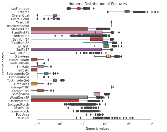
Input[27]:
# Find skewed numerical features
skew_features = all_features[numeric].apply(lambda x: skew(x)).sort_values(ascending=False)	high_skew = skew_features[skew_features > 0.5]
skew_index = high_skew.index	print("There are {} numerical features with Skew > 0.5 :".format(high_skew.shape[0]))
skewness = pd.DataFrame({'Skew' :high_skew})
skew_features.head(10
Output[27]:
There are 25 numerical features with Skew > 0.5 :
MiscVal 21.939672
PoolArea 17.688664
LotArea 13.109495
LowQualFinSF 12.084539
3SsnPorch 11.372080
KitchenAbvGr 4.300550
BsmtFinSF2 4.144503
EnclosedPorch 4.002344
ScreenPorch 3.945101
BsmtHalfBath 3.929996
dtype: float64
使用 scipy 的函数 boxcox1来进行 Box-Cox 转换,将数据正态化
Input[28]:
# Normalize skewed features
for i in skew_index:	all_features[i] = boxcox1p(all_features[i], 	boxcox_normmax(all_features[i] + 1))
Input[29]:
# Let's make sure we handled all the skewed values
sns.set_style("white")
f, ax = plt.subplots(figsize=(8, 7))
ax.set_xscale("log")
ax = sns.boxplot(data=all_features[skew_index] , orient="h", palette="Set1")
ax.xaxis.grid(False)
ax.set(ylabel="Feature names")
ax.set(xlabel="Numeric values")
ax.set(title="Numeric Distribution of Features")
sns.despine(trim=True, left=True) 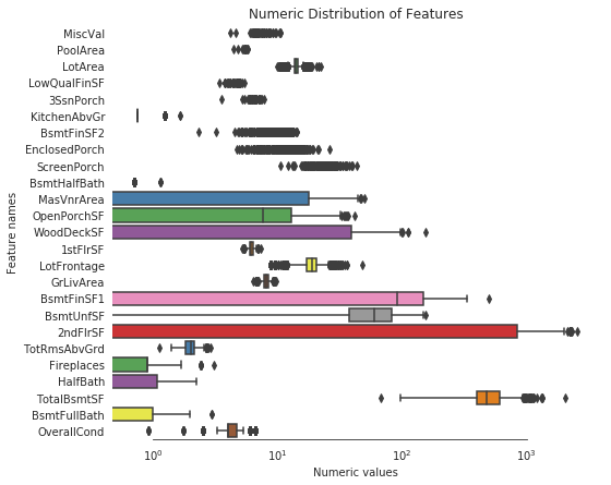
从上图可以看到,所有特征都看上去呈正态分布了。
创建一些有用的特征
机器学习模型对复杂模型的认知较差,因此我们需要用我们的直觉来构建有效的特征,从而帮助模型更加有效的学习。
all_features['BsmtFinType1_Unf'] = 1*(all_features['BsmtFinType1'] == 'Unf')
all_features['HasWoodDeck'] = (all_features['WoodDeckSF'] == 0) * 1
all_features['HasOpenPorch'] = (all_features['OpenPorchSF'] == 0) * 1
all_features['HasEnclosedPorch'] = (all_features['EnclosedPorch'] == 0) * 1
all_features['Has3SsnPorch'] = (all_features['3SsnPorch'] == 0) * 1
all_features['HasScreenPorch'] = (all_features['ScreenPorch'] == 0) * 1
all_features['YearsSinceRemodel'] = all_features['YrSold'].astype(int) - all_features['YearRemodAdd'].astype(int)
all_features['Total_Home_Quality'] = all_features['OverallQual'] + all_features['OverallCond']
all_features = all_features.drop(['Utilities', 'Street', 'PoolQC',], axis=1)
all_features['TotalSF'] = all_features['TotalBsmtSF'] + all_features['1stFlrSF'] + all_features['2ndFlrSF']
all_features['YrBltAndRemod'] = all_features['YearBuilt'] + all_features['YearRemodAdd']	all_features['Total_sqr_footage'] = (all_features['BsmtFinSF1'] + all_features['BsmtFinSF2'] +	all_features['1stFlrSF'] + all_features['2ndFlrSF'])
all_features['Total_Bathrooms'] = (all_features['FullBath'] + (0.5 * all_features['HalfBath']) +	all_features['BsmtFullBath'] + (0.5 * all_features['BsmtHalfBath']))
all_features['Total_porch_sf'] = (all_features['OpenPorchSF'] + all_features['3SsnPorch'] +	all_features['EnclosedPorch'] + all_features['ScreenPorch'] +	all_features['WoodDeckSF'])
all_features['TotalBsmtSF'] = all_features['TotalBsmtSF'].apply(lambda x: np.exp(6) if x <= 0.0 else x)
all_features['2ndFlrSF'] = all_features['2ndFlrSF'].apply(lambda x: np.exp(6.5) if x <= 0.0 else x)
all_features['GarageArea'] = all_features['GarageArea'].apply(lambda x: np.exp(6) if x <= 0.0 else x)
all_features['GarageCars'] = all_features['GarageCars'].apply(lambda x: 0 if x <= 0.0 else x)
all_features['LotFrontage'] = all_features['LotFrontage'].apply(lambda x: np.exp(4.2) if x <= 0.0 else x)
all_features['MasVnrArea'] = all_features['MasVnrArea'].apply(lambda x: np.exp(4) if x <= 0.0 else x)
all_features['BsmtFinSF1'] = all_features['BsmtFinSF1'].apply(lambda x: np.exp(6.5) if x <= 0.0 else x)	all_features['haspool'] = all_features['PoolArea'].apply(lambda x: 1 if x > 0 else 0)
all_features['has2ndfloor'] = all_features['2ndFlrSF'].apply(lambda x: 1 if x > 0 else 0)
all_features['hasgarage'] = all_features['GarageArea'].apply(lambda x: 1 if x > 0 else 0)
all_features['hasbsmt'] = all_features['TotalBsmtSF'].apply(lambda x: 1 if x > 0 else 0)
all_features['hasfireplace'] = all_features['Fireplaces'].apply(lambda x: 1 if x > 0 else 0
特征转换
通过对特征取对数或者平方,可以创造更多的特征,这些操作有利于发掘潜在的有用特征。
def logs(res, ls): m = res.shape[1] for l in ls: res = res.assign(newcol=pd.Series(np.log(1.01+res[l])).values) res.columns.values[m] = l + '_log' m += 1 return res log_features = ['LotFrontage','LotArea','MasVnrArea','BsmtFinSF1','BsmtFinSF2','BsmtUnfSF', 'TotalBsmtSF','1stFlrSF','2ndFlrSF','LowQualFinSF','GrLivArea', 'BsmtFullBath','BsmtHalfBath','FullBath','HalfBath','BedroomAbvGr','KitchenAbvGr', 'TotRmsAbvGrd','Fireplaces','GarageCars','GarageArea','WoodDeckSF','OpenPorchSF', 'EnclosedPorch','3SsnPorch','ScreenPorch','PoolArea','MiscVal','YearRemodAdd','TotalSF'] all_features = logs(all_features, log_featuresdef squares(res, ls): m = res.shape[1] for l in ls: res = res.assign(newcol=pd.Series(res[l]*res[l]).values) res.columns.values[m] = l + '_sq' m += 1 return res squared_features = ['YearRemodAdd', 'LotFrontage_log', 'TotalBsmtSF_log', '1stFlrSF_log', '2ndFlrSF_log', 'GrLivArea_log', 'GarageCars_log', 'GarageArea_log']
all_features = squares(all_features, squared_features)对集合特征进行编码
对集合特征进行数值编码,使得机器学习模型能够处理这些特征。
all_features = pd.get_dummies(all_features).reset_index(drop=True)
all_features.shape
(2917, 379)
all_features.head() 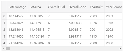
all_features.shape(2917, 379)
# Remove any duplicated column names
all_features = all_features.loc[:,~all_features.columns. duplicated()]
重新创建训练集和测试集
X = all_features.iloc[:len(train_labels), :]
X_test = all_features.iloc[len(train_labels):, :]
X.shape, train_labels.shape, X_test.shape
((1458, 378), (1458,), (1459, 378))
对训练集中的部分特征进行可视化
# Finding numeric features
numeric_dtypes = ['int16', 'int32', 'int64', 'float16', 'float32', 'float64']
numeric = []
for i in X.columns:	if X[i].dtype in numeric_dtypes:	if i in ['TotalSF', 'Total_Bathrooms','Total_porch_sf','haspool','hasgarage','hasbsmt','hasfireplace']:	pass	else:	numeric.append(i)
# visualising some more outliers in the data values
fig, axs = plt.subplots(ncols=2, nrows=0, figsize=(12, 150))
plt.subplots_adjust(right=2)
plt.subplots_adjust(top=2)
sns.color_palette("husl", 8)
for i, feature in enumerate(list(X[numeric]), 1): if(feature=='MiscVal'): break plt.subplot(len(list(numeric)), 3, i) sns.scatterplot(x=feature, y='SalePrice', hue='SalePrice', palette='Blues', data=train) plt.xlabel('{}'.format(feature), size=15,labelpad=12.5) plt.ylabel('SalePrice', size=15, labelpad=12.5) for j in range(2): plt.tick_params(axis='x', labelsize=12) plt.tick_params(axis='y', labelsize=12) plt.legend(loc='best', prop={'size': 10}) plt.show() 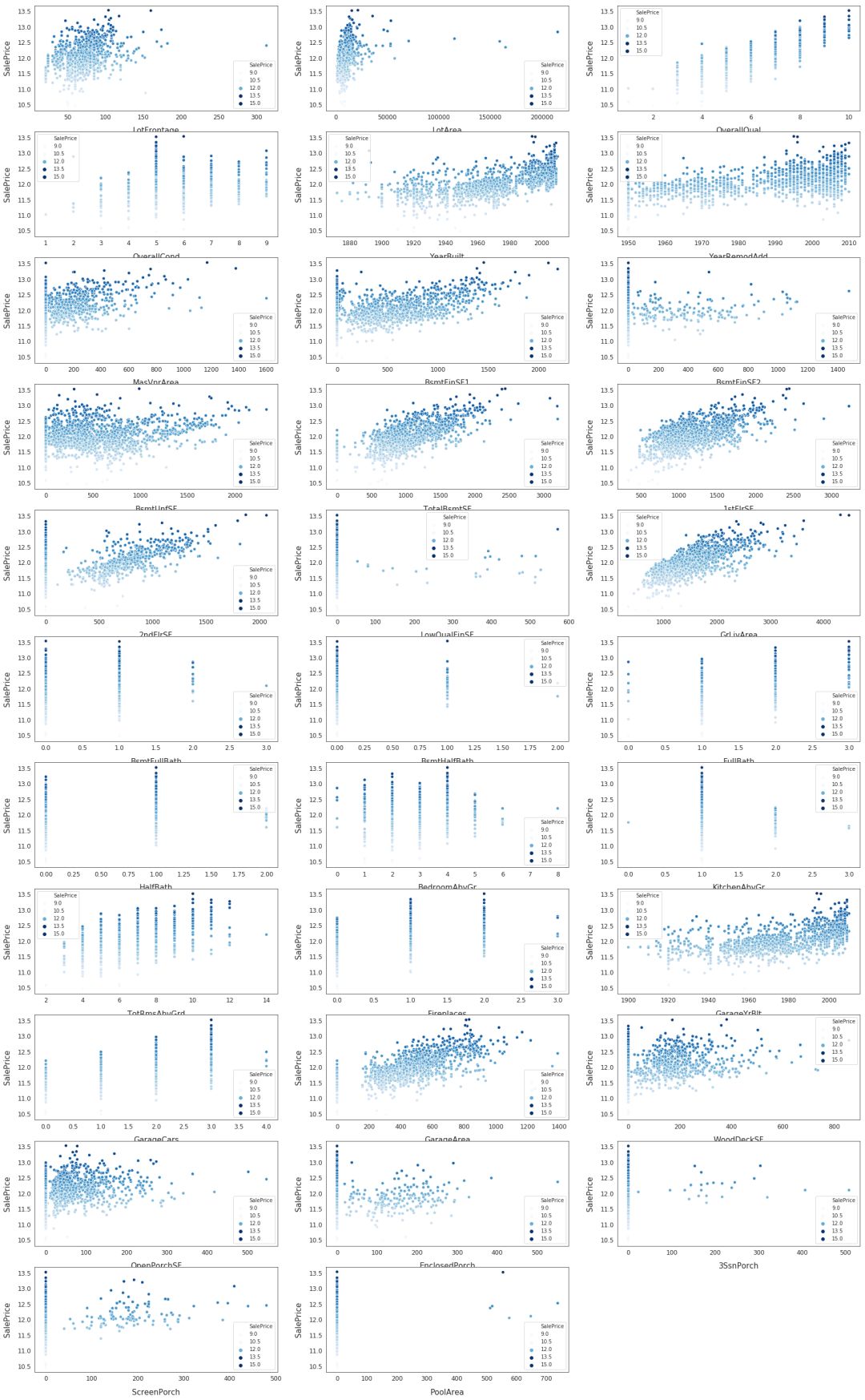
模型训练
模型训练过程中的重要细节
交叉验证:使用12-折交叉验证
模型:在每次交叉验证中,同时训练七个模型(ridge, svr, gradient boosting, random forest, xgboost, lightgbm regressors)
Stacking 方法:使用xgboot训练了元 StackingCVRegressor 学习器
模型融合:所有训练的模型都会在不同程度上过拟合,因此,为了做出最终的预测,将这些模型进行了融合,得到了鲁棒性更强的预测结果
初始化交叉验证,定义误差评估指标
# Setup cross validation folds
kf = KFold(n_splits=12, random_state=42, shuffle=True)
# Define error metrics
def rmsle(y, y_pred): return np.sqrt(mean_squared_error(y, y_pred)) def cv_rmse(model, X=X): rmse = np.sqrt(-cross_val_score(model, X, train_labels, scoring="neg_mean_squared_error", cv=kf)) return (rmse)建立模型
# Light Gradient Boosting Regressor
lightgbm = LGBMRegressor(objective='regression',	num_leaves=6,	learning_rate=0.01,	n_estimators=7000,	max_bin=200,	bagging_fraction=0.8,	bagging_freq=4,	bagging_seed=8,	feature_fraction=0.2,	feature_fraction_seed=8,	min_sum_hessian_in_leaf = 11,	verbose=-1,	random_state=42)	# XGBoost Regressor
xgboost = XGBRegressor(learning_rate=0.01,	n_estimators=6000,	max_depth=4,	min_child_weight=0,	gamma=0.6,	subsample=0.7,	colsample_bytree=0.7,	objective='reg:linear',	nthread=-1,	scale_pos_weight=1,	seed=27,	reg_alpha=0.00006,	random_state=42)	# Ridge Regressor
ridge_alphas = [1e-15, 1e-10, 1e-8, 9e-4, 7e-4, 5e-4, 3e-4, 1e-4, 1e-3, 5e-2, 1e-2, 0.1, 0.3, 1, 3, 5, 10, 15, 18, 20, 30, 50, 75, 100]
ridge = make_pipeline(RobustScaler(), RidgeCV(alphas=ridge_alphas, cv=kf))	# Support Vector Regressor
svr = make_pipeline(RobustScaler(), SVR(C= 20, epsilon= 0.008, gamma=0.0003))	# Gradient Boosting Regressor
gbr = GradientBoostingRegressor(n_estimators=6000,	learning_rate=0.01,	max_depth=4,	max_features='sqrt',	min_samples_leaf=15,	min_samples_split=10,	loss='huber',	random_state=42)	# Random Forest Regressor
rf = RandomForestRegressor(n_estimators=1200,	max_depth=15,	min_samples_split=5,	min_samples_leaf=5,	max_features=None,	oob_score=True,	random_state=42)	# Stack up all the models above, optimized using xgboost
stack_gen = StackingCVRegressor(regressors=(xgboost, lightgbm, svr, ridge, gbr, rf),	meta_regressor=xgboost,	use_features_in_secondary=True)
训练模型
计算每个模型的交叉验证的得分
scores = {}	score = cv_rmse(lightgbm)
print("lightgbm: {:.4f} ({:.4f})".format(score.mean(), score.std()))
scores['lgb'] = (score.mean(), score.std())
lightgbm: 0.1159 (0.0167)
score = cv_rmse(xgboost)
print("xgboost: {:.4f} ({:.4f})".format(score.mean(), score.std()))
scores['xgb'] = (score.mean(), score.std())
xgboost: 0.1364 (0.0175)
score = cv_rmse(svr)
print("SVR: {:.4f} ({:.4f})".format(score.mean(), score.std()))
scores['svr'] = (score.mean(), score.std())
SVR: 0.1094 (0.0200)
score = cv_rmse(ridge)
print("ridge: {:.4f} ({:.4f})".format(score.mean(), score.std()))
scores['ridge'] = (score.mean(), score.std())
ridge: 0.1101 (0.0161)
score = cv_rmse(rf)
print("rf: {:.4f} ({:.4f})".format(score.mean(), score.std()))
scores['rf'] = (score.mean(), score.std())
rf: 0.1366 (0.0188
score = cv_rmse(gbr)
print("gbr: {:.4f} ({:.4f})".format(score.mean(), score.std()))
scores['gbr'] = (score.mean(), score.std())
gbr: 0.1121 (0.0164)
拟合模型
print('stack_gen')
stack_gen_model = stack_gen.fit(np.array(X), np.array(train_labels))
stack_gen
print('lightgbm')
lgb_model_full_data = lightgbm.fit(X, train_labels)
lightgbm
print('xgboost')
xgb_model_full_data = xgboost.fit(X, train_labels)
xgboost
print('Svr')
svr_model_full_data = svr.fit(X, train_labels)
Svr
print('Ridge')
ridge_model_full_data = ridge.fit(X, train_labels)
Ridge
print('RandomForest')
rf_model_full_data = rf.fit(X, train_labels)
RandomForest
print('GradientBoosting')
gbr_model_full_data = gbr.fit(X, train_labels)
GradientBoosting
融合各个模型,并进行最终预测
# Blend models in order to make the final predictions more robust to overfitting
def blended_predictions(X):	return ((0.1 * ridge_model_full_data.predict(X)) + \	(0.2 * svr_model_full_data.predict(X)) + \	(0.1 * gbr_model_full_data.predict(X)) + \	(0.1 * xgb_model_full_data.predict(X)) + \	(0.1 * lgb_model_full_data.predict(X)) + \	(0.05 * rf_model_full_data.predict(X)) + \	(0.35 * stack_gen_model.predict(np.array(X))))
# Get final precitions from the blended model
blended_score = rmsle(train_labels, blended_predictions(X))
scores['blended'] = (blended_score, 0)
print('RMSLE score on train data:')
print(blended_score)
RMSLE score on train data:
0.07537440195302639
各模型性能比较
# Plot the predictions for each model
sns.set_style("white")
fig = plt.figure(figsize=(24, 12))	ax = sns.pointplot(x=list(scores.keys()), y=[score for score, _ in scores.values()], markers=['o'], linestyles=['-'])
for i, score in enumerate(scores.values()):	ax.text(i, score[0] + 0.002, '{:.6f}'.format(score[0]), horizontalalignment='left', size='large', color='black', weight='semibold')	plt.ylabel('Score (RMSE)', size=20, labelpad=12.5)
plt.xlabel('Model', size=20, labelpad=12.5)
plt.tick_params(axis='x', labelsize=13.5)
plt.tick_params(axis='y', labelsize=12.5) plt.title('Scores of Models', size=20) plt.sho 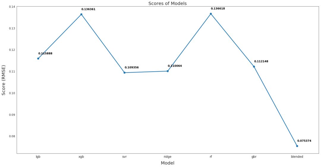
从上图可以看出,融合后的模型性能最好,RMSE 仅为 0.075,该融合模型用于最终预测。
提交预测结果
# Read in sample_submission dataframe
submission = pd.read_csv("../input/house-prices-advanced-regression-techniques/sample_submission.csv")
submission.shape
(1459, 2)
# Append predictions from blended models
submission.iloc[:,1] = np.floor(np.expm1(blended_predictions(X_test)))	# Fix outleir predictions
q1 = submission['SalePrice'].quantile(0.0045)
q2 = submission['SalePrice'].quantile(0.99)
submission['SalePrice'] = submission['SalePrice'].apply(lambda x: x if x > q1 else x*0.77)
submission['SalePrice'] = submission['SalePrice'].apply(lambda x: x if x < q2 else x*1.1)
submission.to_csv("submission_regression1.csv", index=False)
# Scale predictions
submission['SalePrice'] *= 1.001619
submission.to_csv("submission_regression2.csv", index=False)原文链接:
https://www.kaggle.com/lavanyashukla01/how-i-made-top-0-3-on-a-kaggle-competition
(*本文为 AI科技大本营翻译文章,转载请联系 1092722531)
◆
精彩推荐
◆
“只讲技术,拒绝空谈!”2019 AI开发者大会将于9月6日-7日在北京举行,这一届AI开发者大会有哪些亮点?一线公司的大牛们都在关注什么?AI行业的风向是什么?2019 AI开发者大会,倾听大牛分享,聚焦技术实践,和万千开发者共成长。
目前,大会盲订票限量发售中~扫码购票,领先一步!

推荐阅读
干货 | 20个教程,掌握时间序列的特征分析(附代码)
从发展滞后到不断突破,NLP已成为AI又一燃爆点?
长点心吧年轻人,利率不是这么算的!我用Python告诉你亏了多少!
一文看懂数据清洗:缺失值、异常值和重复值的处理
Libra 骗局来了! 受害者会是你吗?
那个裸辞的程序员,后来怎么样了?
FreeWheel是一家怎样的公司?| 人物志
Mac 被曝存在恶意漏洞:黑客可随意调动摄像头,波及四百万用户!
文末送书啦!| Device Mapper,那些你不知道的Docker核心技术
 你点的每个“在看”,我都认真当成了喜欢