pandas是基于NumPy的一种数据分析工具,在机器学习任务中,我们首先需要对数据进行清洗和编辑等工作,pandas库大大简化了我们的工作量,熟练并掌握pandas常规用法是正确构建机器学习模型的第一步。
1. 安装
最常用的方法是通过Anaconda安装,在终端或命令符输入如下命令安装:
conda install pandas
若未安装Anaconda,使用Python自带的包管理工具pip来安装:
pip install pandas
2. 导入pandas库和查询相应的版本信息
import numpy as np   # pandas和numpy常常结合在一起使用,导入numpy库
import pandas as pd  # 导入pandas库print(pd.__version__) # 打印pandas版本信息#> 0.23.4
3. pandas数据类型
pandas包含两种数据类型:series和dataframe。
series是一种一维数据结构,每一个元素都带有一个索引,与一维数组的含义相似,其中索引可以为数字或字符串。series结构名称:
|索引列|数据列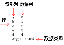
dataframe是一种二维数据结构,数据以表格形式(与excel类似)存储,有对应的行和列。dataframe结构名称: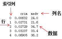
4. series教程
- 从列表,数组,字典构建series
mylist = list('abcedfghijklmnopqrstuvwxyz')   # 列表
myarr = np.arange(26)	                      # 数组
mydict = dict(zip(mylist, myarr))             # 字典# 构建方法ser1 = pd.Series(mylist)ser2 = pd.Series(myarr)ser3 = pd.Series(mydict)print(ser3.head())                 # 打印前5个数据#>  a    0b    1c    2d    4e    3dtype:int64
- 使series的索引列转化为dataframe的列
mylist = list('abcedfghijklmnopqrstuvwxyz')
myarr = np.arange(26)
mydict = dict(zip(mylist, myarr))
ser = pd.Series(mydict)# series转换为dataframe
df = ser.to_frame()
# 索引列转换为dataframe的列df.reset_index(inplace=True)
print(df.head())#>	  index  00     a  01     b  12     c  23     e  34     d  4
- 结合多个series组成dataframe
# 构建series1
ser1 = pd.Series(list('abcedfghijklmnopqrstuvwxyz'))
# 构建series2
ser2 = pd.Series(np.arange(26))# 方法1,axis=1表示列拼接,0表示行拼接
df = pd.concat([ser1, ser2], axis=1)# 与方法1相比,方法2设置了列名df = pd.DataFrame({'col1': ser1, 'col2': ser2})print(df.head())#>	  col1  col20    a     01    b     12    c     23    e     34    d     4
- 命名列索引的名称
ser = pd.Series(list('abcedfghijklmnopqrstuvwxyz'))\# 命名索引列名称
ser.name = 'alphabets'
\# 显示前5行数据ser.head()#>	0    a1    b2    c3    e4    dName: alphabets, dtype: object
- 如何获得series对象A中不包含series对象B的元素
ser1 = pd.Series([1, 2, 3, 4, 5])
ser2 = pd.Series([4, 5, 6, 7, 8])\# 返回ser1不包含ser2的布尔型series
ser3=~ser1.isin(ser2)
\# 获取ser不包含ser2的元素ser1[ser3]#>	0    11    22    3dtype: int64
- 如何获得seriesA和seriesB不相同的项
ser1 = pd.Series([1, 2, 3, 4, 5])
ser2 = pd.Series([4, 5, 6, 7, 8])\# 求ser1和ser2的并集
ser_u = pd.Series(np.union1d(ser1, ser2))
# 求ser1和ser2的交集
ser_i = pd.Series(np.intersect1d(ser1, ser2))
\# ser_i在ser_u的补集就是ser1和ser2不相同的项ser_u[~ser_u.isin(ser_i)]#>	0    11    22    35    66    77    8dtype: int64
- 获得数值series的四分位值
\# 设置随机数种子
state = np.random.RandomState(100)
\# 从均值为5标准差为25的正态分布随机抽取5个点构成series
ser = pd.Series(state.normal(10, 5, 25))
\# 求ser的四分位数np.percentile(ser, q=[0, 25, 50, 75, 100])#> array([ 1.25117263,  7.70986507, 10.92259345, 13.36360403, 18.0949083 ])
- 获得series中单一项的频率计数
#从0~7随机抽取30个列表值,组成series
ser = pd.Series(np.take(list('abcdefgh'), np.random.randint(8, size=30)))
# 对该series进行计数ser.value_counts()#>	d    8g    6b    6a    5e    2h    2f    1dtype: int64
- 保留series中前两个频次最多的项,其他项替换为‘other’
np.random.RandomState(100)
\# 从1~4均匀采样12个点组成seriesser = pd.Series(np.random.randint(1, 5, [12]))# 除前两行索引对应的值不变,后几行索引对应的值为Otherser[~ser.isin(ser.value_counts().index[:2])] = 'Other'ser#>	0     Other1         42         23         24         45     Other6     Other7     Other8         49         410        411        2dtype: object
- 对数值series分成10个相同数目的组
换个角度理解,对数值series离散化成10个类别(categorical)值
ser = pd.Series(np.random.random(20))\# 离散化10个类别值,只显示前5行的数据pd.qcut(ser, q=[0, .10, .20, .3, .4, .5, .6, .7, .8, .9, 1], labels=['1st', '2nd', '3rd', '4th', '5th', '6th', '7th', '8th', '9th', '10th']).head()#>0 3rd1 1st2 6th3 6th4 9thdtype: categoryCategories (10, object): [1st < 2nd < 3rd < 4th ... 7th < 8th < 9th < 10th]
- 使numpy数组转化为给定形状的dataframe
ser = pd.Series(np.random.randint(1, 10, 35))
\# serier类型转换numpy类型,然后重构df = pd.DataFrame(ser.values.reshape(7,5))print(df)#>	   0  1  2  3  40  1  2  1  2  51  1  2  4  5  22  1  3  3  2  83  8  6  4  9  64  2  1  1  8  55  3  2  8  5  66  1  5  5  4  6
- 找到series的值是3的倍数的位置
ser = pd.Series(np.random.randint(1, 10, 7))
print(ser)# 获取值是3倍数的索引np.argwhere(ser % 3==0)#>	0    61    82    63    74    65    26    4dtype: int64#>	array([[0],[2],[4]])
- 获取series中给定索引的元素(items)
ser = pd.Series(list('abcdefghijklmnopqrstuvwxyz'))
index = [0, 4, 8, 14, 20]# 获取指定索引的元素ser.take(index)#>	0     a4     e8     i14    o20    udtype: object
- 垂直和水平的拼接series
ser1 = pd.Series(range(5))
ser2 = pd.Series(list('abcde'))# 垂直拼接
df = pd.concat([ser1, ser2], axis=0)# 水平拼接df = pd.concat([ser1, ser2], axis=1)print(df)#>	   0  10  0  a1  1  b2  2  c3  3  d4  4  e
- 获取series对象A中包含series对象B元素的位置
# ser1必须包含ser2,否则会报错
ser1 = pd.Series([10, 9, 6, 5, 3, 1, 12, 8, 13])
ser2 = pd.Series([1, 3, 10, 13])# 方法 1
[np.where(i == ser1)[0].tolist()[0] for i in ser2]# 方法 2
[pd.Index(ser1).get_loc(i) for i in ser2]#> [5, 4, 0, 8]
16.如何计算series之间的均方差
truth = pd.Series(range(10))
pred = pd.Series(range(10)) + np.random.random(10)# 均方差
np.mean((truth-pred)**2)#> 0.25508722434194103
- 使series中每个元素的首字母为大写
# series的元素为str类型
ser = pd.Series(['how', 'to', 'kick', 'ass?'])# 方法 1
ser.map(lambda x: x.title())# 方法 2 ,字符串相加
ser.map(lambda x: x[0].upper() + x[1:])# 方法 3pd.Series([i.title() for i in ser])#>	0     How1      To2    Kick3    Ass?dtype: object
- 计算series中每个元素的字符串长度
ser = pd.Series(['how', 'to', 'kick', 'ass?'])# 方法ser.map(lambda x: len(x))#> 0 31 22 43 4dtype: int64
- 计算series的一阶导和二阶导
ser = pd.Series([1, 3, 6, 10, 15, 21, 27, 35])# 求一阶导并转化为列表类型
print(ser.diff().tolist())
# 求二阶导并转化为列表类型print(ser.diff().diff().tolist())#>	[nan, 2.0, 3.0, 4.0, 5.0, 6.0, 6.0, 8.0][nan, nan, 1.0, 1.0, 1.0, 1.0, 0.0, 2.0]
- 将一系列日期字符串转换为timeseries
ser = pd.Series(['01 Jan 2010', '02-02-2011', '20120303', '2013/04/04', '2014-05-05', '2015-06-06T12:20'])pd.to_datetime(ser)#> 0 2010-01-01 00:00:001 2011-02-02 00:00:002 2012-03-03 00:00:003 2013-04-04 00:00:004 2014-05-05 00:00:005 2015-06-06 12:20:00dtype: datetime64[ns]
- 从一个series中获取至少包含两个元音的元素
ser = pd.Series(['Apple', 'Orange', 'Plan', 'Python', 'Money'])# 方法from collections import Counter# Counter是一个类字典类型,键是元素值,值是元素出现的次数,满足条件的元素返回Truemask = ser.map(lambda x: sum([Counter(x.lower()).get(i, 0) for i in list('aeiou')]) >= 2)ser[mask]#> 0 Apple1 Orange4 Moneydtype: object
- 计算根据另一个series分组后的series均值
fruit = pd.Series(np.random.choice(['apple', 'banana', 'carrot'], 10))weights = pd.Series(np.linspace(1, 10, 10))\# 根据fruit对weight分组weightsGrouped = weights.groupby(fruit)print(weightsGrouped.indices)\# 对分组后series求每个索引的平均值weightsGrouped.mean()#> {'apple': array([0, 3], dtype=int64), 'banana': array([1, 2, 4, 8],dtype=int64), 'carrot': array([5, 6, 7, 9], dtype=int64)}#> apple 2.50banana 4.75carrot 7.75dtype: float64
- 计算两个series之间的欧氏距离
p = pd.Series([1, 2, 3, 4, 5, 6, 7, 8, 9, 10])q = pd.Series([10, 9, 8, 7, 6, 5, 4, 3, 2, 1])\# 方法1sum((p - q)**2)**.5\# 方法2np.linalg.norm(p-q)#> 18.16590212458495
- 在数值series中找局部最大值
局部最大值对应二阶导局部最小值
ser = pd.Series([2, 10, 3, 4, 9, 10, 2, 7, 3])\# 二阶导dd = np.diff(np.sign(np.diff(ser)))\# 二阶导的最小值对应的值为最大值,返回最大值的索引peak_locs = np.where(dd == -2)[0] + 1peak_locs#> array([1, 5, 7], dtype=int64)
- 如何用最少出现的字符替换空格符
my_str = 'dbc deb abed gade'# 方法
ser = pd.Series(list('dbc deb abed gade'))
# 统计元素的频数
freq = ser.value_counts()
print(freq)
# 求最小频数的字符
least_freq = freq.dropna().index[-1]
# 替换
"".join(ser.replace(' ', least_freq))#>	d    43b    3e    3a    2c    1g    1dtype: int64#>	'dbcgdebgabedggade'
- 计算数值series的自相关系数
ser = pd.Series(np.arange(20) + np.random.normal(1, 10, 20))# 求series的自相关系数,i为偏移量
autocorrelations = [ser.autocorr(i).round(2) for i in range(11)]
print(autocorrelations[1:])
# 选择最大的偏移量
print('Lag having highest correlation: ', np.argmax(np.abs(autocorrelations[1:]))+1)#>	[0.33, 0.41, 0.48, 0.01, 0.21, 0.16, -0.11, 0.05, 0.34, -0.24]
#>	Lag having highest correlation:  3
- 对series进行算术运算操作
# 如何对series之间进行算法运算
import pandas as pd
series1 = pd.Series([3,4,4,4],['index1','index2','index3','index4'])
series2 = pd.Series([2,2,2,2],['index1','index2','index33','index44'])
# 加法
series_add = series1 + series2
print(series_add)
# 减法
series_minus = series1 - series2
# series_minus
# 乘法
series_multi = series1 * series2
# series_multi
# 除法
series_div = series1/series2
series_div
series是基于索引进行算数运算操作的,pandas会根据索引对数据进行运算,若series之间有不同的索引,对应的值就为Nan。结果如下:
#加法:
index1     5.0
index2     6.0
index3     NaN
index33    NaN
index4     NaN
index44    NaN
dtype: float64
#除法:
index1     1.5
index2     2.0
index3     NaN
index33    NaN
index4     NaN
index44    NaN
dtype: float64
5. dataframe教程
- 从csv文件只读取前几行的数据
# 只读取前2行和指定列的数据
df = pd.read_csv('https://raw.githubusercontent.com/selva86/datasets/master/Cars93_miss.csv',nrows=2,usecols=['Model','Length'])
df#>		Model	Length
0	Integra	177
1	Legend	195
- 从csv文件中每隔n行来创建dataframe
# 每隔50行读取一行数据
df = pd.read_csv('https://raw.githubusercontent.com/selva86/datasets/master/BostonHousing.csv', chunksize=50)
df2 = pd.DataFrame()
for chunk in df:# 获取seriesdf2 = df2.append(chunk.iloc[0,:])#显示前5行
print(df2.head())#>	                  crim    zn  indus chas                  nox     rm   age  \0              0.21977   0.0   6.91    0  0.44799999999999995  5.602  62.0   1               0.0686   0.0   2.89    0                0.445  7.416  62.5   2   2.7339700000000002   0.0  19.58    0                0.871  5.597  94.9   3               0.0315  95.0   1.47    0  0.40299999999999997  6.975  15.3   4  0.19072999999999998  22.0   5.86    0                0.431  6.718  17.5   dis rad  tax ptratio       b  lstat  medv  0  6.0877   3  233    17.9   396.9   16.2  19.4  1  3.4952   2  276    18.0   396.9   6.19  33.2  2  1.5257   5  403    14.7  351.85  21.45  15.4  3  7.6534   3  402    17.0   396.9   4.56  34.9  4  7.8265   7  330    19.1  393.74   6.56  26.2
- 改变导入csv文件的列值
改变列名‘medv’的值,当列值≤25时,赋值为‘Low’;列值>25时,赋值为‘High’.
# 使用converters参数,改变medv列的值
df = pd.read_csv('https://raw.githubusercontent.com/selva86/datasets/master/BostonHousing.csv', converters={'medv': lambda x: 'High' if float(x) > 25 else 'Low'})
print(df.head())#>	        b  lstat  medv0  396.90   4.98   Low  1  396.90   9.14   Low  2  392.83   4.03  High  3  394.63   2.94  High  4  396.90   5.33  High
- 从csv文件导入指定的列
# 导入指定的列:crim和medv
df = pd.read_csv('https://raw.githubusercontent.com/selva86/datasets/master/BostonHousing.csv', usecols=['crim', 'medv'])
# 打印前四行dataframe信息
print(df.head())#>	      crim  medv0  0.00632  24.01  0.02731  21.62  0.02729  34.73  0.03237  33.44  0.06905  36.2
- 得到dataframe的行,列,每一列的类型和相应的描述统计信息
df = pd.read_csv('https://raw.githubusercontent.com/selva86/datasets/master/Cars93_miss.csv')#  打印dataframe的行和列
print(df.shape)# 打印dataframe每列元素的类型显示前5行
print(df.dtypes.head())# 统计各类型的数目,方法1
print(df.get_dtype_counts())
# 统计各类型的数目,方法2
# print(df.dtypes.value_counts())# 描述每列的统计信息,如std,四分位数等
df_stats = df.describe()
# dataframe转化数组
df_arr = df.values
# 数组转化为列表
df_list = df.values.tolist()#>	(93, 27)Manufacturer     objectModel            objectType             objectMin.Price       float64Price           float64dtype: objectfloat64    18object      9dtype: int64
- 获取给定条件的行和列
import numpy as np
df = pd.read_csv('https://raw.githubusercontent.com/selva86/datasets/master/Cars93_miss.csv')
# print(df)
# 获取最大值的行和列
row, col = np.where(df.values == np.max(df.Price))
# 行和列获取最大值
print(df.iat[row[0], col[0]])
df.iloc[row[0], col[0]]# 行索引和列名获取最大值
df.at[row[0], 'Price']
df.get_value(row[0], 'Price')#>	61.9
- 重命名dataframe的特定列
df1 = pd.DataFrame(data=np.array([[18,50],[19,51],[20,55]]),index=['man1','man2','man3'],columns=['age','weight'])
print(df1)
# 修改列名
print("\nchange columns :\n")
#方法1
df1.rename(columns={'weight':'stress'})
#方法2
df1.columns.values[1] = 'stress'
print(df1)#>	      age  weightman1   18      50man2   19      51man3   20      55change columns :age  stressman1   18      50man2   19      51man3   20      55
- 如何检查dataframe中是否有缺失值
df = pd.read_csv('https://raw.githubusercontent.com/selva86/datasets/master/Cars93_miss.csv')# 若有缺失值,则为Ture
df.isnull().values.any()#>	True
9. 如何统计dataframe的每列中缺失值的个数
df = pd.read_csv('https://raw.githubusercontent.com/selva86/datasets/master/Cars93_miss.csv')# 获取每列的缺失值个数
n_missings_each_col = df.apply(lambda x: x.isnull().sum())
print(n_missings_each_col.head())#>	Manufacturer    4Model           1Type            3Min.Price       7Price           2dtype: int64
- 用平均值替换相应列的缺失值
df = pd.read_csv('https://raw.githubusercontent.com/selva86/datasets/master/Cars93_miss.csv',nrows=10)
print(df[['Min.Price','Max.Price']].head())
# 平均值替换缺失值
df_out = df[['Min.Price', 'Max.Price']] = df[['Min.Price', 'Max.Price']].apply(lambda x: x.fillna(x.mean()))
print(df_out.head())#>	   Min.Price  Max.Price0       12.9       18.81       29.2       38.72       25.9       32.33        NaN       44.64        NaN        NaN#>	   Min.Price  Max.Price0       12.9       18.81       29.2       38.72       25.9       32.33       23.0       44.64       23.0       29.9
- 用全局变量作为apply函数的附加参数处理指定的列
df = pd.read_csv('https://raw.githubusercontent.com/selva86/datasets/master/Cars93_miss.csv')
print(df[['Min.Price', 'Max.Price']].head())
# 全局变量
d = {'Min.Price': np.nanmean, 'Max.Price': np.nanmedian}
# 列名Min.Price的缺失值用平均值代替,Max.Price的缺失值用中值代替
df[['Min.Price', 'Max.Price']] = df[['Min.Price', 'Max.Price']].apply(lambda x, d: x.fillna(d[x.name](x)), args=(d, ))
print(df[['Min.Price', 'Max.Price']].head())#>	   Min.Price  Max.Price0       12.9       18.81       29.2       38.72       25.9       32.33        NaN       44.64        NaN        NaN#>	   Min.Price  Max.Price0  12.900000      18.801  29.200000      38.702  25.900000      32.303  17.118605      44.604  17.118605      19.15
- 以dataframe的形式选择特定的列
df = pd.DataFrame(np.arange(20).reshape(-1, 5), columns=list('abcde'))
# print(df)# 以dataframe的形式选择特定的列
type(df[['a']])
type(df.loc[:, ['a']])
print(type(df.iloc[:, [0]]))# 以series的形式选择特定的列
type(df.a)
type(df['a'])
type(df.loc[:, 'a'])
print(type(df.iloc[:, 1]))#>	<class 'pandas.core.frame.DataFrame'><class 'pandas.core.series.Series'>
- 改变dataframe中的列顺序
df = pd.DataFrame(np.arange(20).reshape(-1, 5), columns=list('abcde'))print(df)
# 交换col1和col2
def switch_columns(df, col1=None, col2=None):colnames = df.columns.tolist()i1, i2 = colnames.index(col1), colnames.index(col2)colnames[i2], colnames[i1] = colnames[i1], colnames[i2]return df[colnames]df1 = switch_columns(df, 'a', 'c')
print(df1)#>	    a   b   c   d   e0   0   1   2   3   41   5   6   7   8   92  10  11  12  13  143  15  16  17  18  19
#>	    c   b   a   d   e0   2   1   0   3   41   7   6   5   8   92  12  11  10  13  143  17  16  15  18  19
- 格式化dataframe的值
df = pd.DataFrame(np.random.random(4)**10, columns=['random'])
print(df)
# 显示小数点后四位
df.apply(lambda x: '%.4f' % x, axis=1)
print(df)#>	         random0  3.539348e-041  3.864140e-102  2.973575e-023  1.414061e-01
#>	         random0  3.539348e-041  3.864140e-102  2.973575e-023  1.414061e-01
- 将dataframe中的所有值以百分数的格式表示
df = pd.DataFrame(np.random.random(4), columns=['random'])# 格式化为小数点后两位的百分数
out = df.style.format({'random': '{0:.2%}'.format,
})out#>		random0	48.54%1	91.51%2	90.83%3	20.45%
- 从dataframe中每隔n行构建dataframe
df = pd.read_csv('https://raw.githubusercontent.com/selva86/datasets/master/Cars93_miss.csv')# 每隔20行读dataframe数据
print(df.iloc[::20, :][['Manufacturer', 'Model', 'Type']])#>	   Manufacturer    Model     Type0         Acura  Integra    Small20     Chrysler  LeBaron  Compact40        Honda  Prelude   Sporty60      Mercury   Cougar  Midsize80       Subaru   Loyale    Small
- 得到列中前n个最大值对应的索引
df = pd.DataFrame(np.random.randint(1, 15, 15).reshape(5,-1), columns=list('abc'))
print(df)
# 取'a'列前3个最大值对应的行
n = 5
df['a'].argsort()[::-1].iloc[:3]#>	    a   b   c0   5   5   21  12   7   12   5   2  123   5  14  124   1  13  13#>	4    13    32    2Name: a, dtype: int64
- 获得dataframe行的和大于100的最末n行索引
df = pd.DataFrame(np.random.randint(10, 40, 16).reshape(-1, 4))
print(df)
# dataframe每行的和
rowsums = df.apply(np.sum, axis=1)# 选取大于100的最末两行索引
# last_two_rows = df.iloc[np.where(rowsums > 100)[0][-2:], :]
nline = np.where(rowsums > 100)[0][-2:]
nline#>	    0   1   2   30  19  34  15  121  38  35  14  262  39  32  18  203  28  27  36  38#>	array([2, 3], dtype=int64)
- 从series中查找异常值并赋值
ser = pd.Series(np.logspace(-2, 2, 30))# 小于low_per分位的数赋值为low,大于low_per分位的数赋值为high
def cap_outliers(ser, low_perc, high_perc):low, high = ser.quantile([low_perc, high_perc])print(low_perc, '%ile: ', low, '|', high_perc, '%ile: ', high)ser[ser < low] = lowser[ser > high] = highreturn(ser)capped_ser = cap_outliers(ser, .05, .95)#>	0.05 %ile:  0.016049294076965887 | 0.95 %ile:  63.876672220183934
- 交换dataframe的两行
df = pd.DataFrame(np.arange(9).reshape(3, -1))
print(df)
# 函数
def swap_rows(df, i1, i2):a, b = df.iloc[i1, :].copy(), df.iloc[i2, :].copy()# 通过iloc换行df.iloc[i1, :], df.iloc[i2, :] = b, areturn df# 2和3行互换
print(swap_rows(df, 1, 2))#>	   0  1  20  0  1  21  3  4  52  6  7  8#>	   0  1  20  0  1  21  6  7  82  3  4  5
- 倒转dataframe的行
df = pd.DataFrame(np.arange(9).reshape(3, -1))
print(df)# 方法 1
df.iloc[::-1, :]# 方法 2
print(df.loc[df.index[::-1], :])#>	   0  1  20  0  1  21  3  4  52  6  7  8#>	   0  1  22  6  7  81  3  4  50  0  1  2
- 对分类变量进行one-hot编码
df = pd.DataFrame(np.arange(25).reshape(5,-1), columns=list('abcde'))
print(df)
# 对列'a'进行onehot编码
df_onehot = pd.concat([pd.get_dummies(df['a']), df[list('bcde')]], axis=1)
print(df_onehot)#>	    a   b   c   d   e0   0   1   2   3   41   5   6   7   8   92  10  11  12  13  143  15  16  17  18  194  20  21  22  23  24#>	   0  5  10  15  20   b   c   d   e0  1  0   0   0   0   1   2   3   41  0  1   0   0   0   6   7   8   92  0  0   1   0   0  11  12  13  143  0  0   0   1   0  16  17  18  194  0  0   0   0   1  21  22  23  24
- 获取dataframe行方向上最大值个数最多的列
df = pd.DataFrame(np.random.randint(1,100, 9).reshape(3, -1))
print(df)
# 获取每列包含行方向上最大值的个数
count_series = df.apply(np.argmax, axis=1).value_counts()
print(count_series)
# 输出行方向最大值个数最多的列的索引
print('Column with highest row maxes: ', count_series.index[0])#>	    0   1   20  46  31  341  38  13   62   1  18  15#>统计列的最大值的个数0    21    1dtype: int64#>	Column with highest row maxes:  0
- 得到列之间最大的相关系数
df = pd.DataFrame(np.random.randint(1,100, 16).reshape(4, -1), columns=list('pqrs'), index=list('abcd'))
# df
print(df)
# 得到四个列的相关系数
abs_corrmat = np.abs(df.corr())
print(abs_corrmat)
# 得到每个列名与其他列的最大相关系数
max_corr = abs_corrmat.apply(lambda x: sorted(x)[-2])
# 显示每列与其他列的相关系数
print('Maximum Correlation possible for each column: ', np.round(max_corr.tolist(), 2))#>	    p   q   r   sa  59  99   1  34b  89  60  97  40c  43  35  14   6d  70  59  30  53
#>	          p         q         r         sp  1.000000  0.200375  0.860051  0.744529q  0.200375  1.000000  0.236619  0.438541r  0.860051  0.236619  1.000000  0.341399s  0.744529  0.438541  0.341399  1.000000#>	Maximum Correlation possible for each column:  [0.86 0.44 0.86 0.74]
- 创建包含每行最小值与最大值比例的列
df = pd.DataFrame(np.random.randint(1,100, 9).reshape(3, -1))
print(df)
# 方法1:axis=1表示行方向,
min_by_max = df.apply(lambda x: np.min(x)/np.max(x), axis=1)# 方法2
min_by_max = np.min(df, axis=1)/np.max(df, axis=1)min_by_max#>	    0   1   20  81  68  591  45  73  232  20  22  69#>	0    0.7283951    0.3150682    0.289855dtype: float64
- 创建包含每行第二大值的列
df = pd.DataFrame(np.random.randint(1,100, 9).reshape(3, -1))
print(df)
# 行方向上取第二大的值组成series
out = df.apply(lambda x: x.sort_values().unique()[-2], axis=1)
# 构建dataframe新的列
df['penultimate'] = out
print(df)#>	    0   1   20  28  77   11  43  19  692  29  30  72#>	    0   1   2  penultimate0  28  77   1           281  43  19  69           432  29  30  72           30
- 归一化dataframe的所有列
df = pd.DataFrame(np.random.randint(1,100, 80).reshape(8, -1))# 正态分布归一化
out1 = df.apply(lambda x: ((x - x.mean())/x.std()).round(2))
print('Solution Q1\n',out1)# 线性归一化
out2 = df.apply(lambda x: ((x.max() - x)/(x.max() - x.min())).round(2))
print('Solution Q2\n', out2)
- 计算每一行与下一行的相关性
df = pd.DataFrame(np.random.randint(1,100, 25).reshape(5, -1))# 行与行之间的相关性
[df.iloc[i].corr(df.iloc[i+1]).round(2) for i in range(df.shape[0])[:-1]]
- 用0赋值dataframe的主对角线和副对角线
df = pd.DataFrame(np.random.randint(1,100, 25).reshape(5, -1))
print(df)
# zhu
for i in range(df.shape[0]):df.iat[i, i] = 0df.iat[df.shape[0]-i-1, i] = 0
print(df)#>	    0   1   2   3   40  51  35  71  71  791  78  25  71  85  442  90  97  72  14   43  27  91  37  25  484   1  26  68  70  20#>	    0   1   2   3   40   0  35  71  71   01  78   0  71   0  442  90  97   0  14   43  27   0  37   0  484   0  26  68  70   0
- 得到按列分组的dataframe的平均值和标准差
df = pd.DataFrame({'col1': ['apple', 'banana', 'orange'] * 2,'col2': np.random.randint(0,15,6),'col3': np.random.randint(0, 15, 6)})
print(df)
# 按列col1分组后的平均值
df_grouped_mean = df.groupby(['col1']).mean()
print(df_grouped_mean)
# 按列col1分组后的标准差
df_grouped_std = df.groupby(['col1']).mean()
print(df_grouped_std)#>	     col1  col2  col30   apple     2    141  banana    11     82  orange     8    103   apple     5     24  banana     6    125  orange    11    13
#>	        col2  col3col1              apple    3.5   8.0banana   8.5  10.0orange   9.5  11.5
#>	        col2  col3col1              apple    3.5   8.0banana   8.5  10.0orange   9.5  11.5
- 如何得到按列分组后另一列的第n大的值
df = pd.DataFrame({'fruit': ['apple', 'banana', 'orange'] * 2,'taste': np.random.rand(6),'price': np.random.randint(0, 15, 6)})print(df)# teste列按fruit分组
df_grpd = df['taste'].groupby(df.fruit)
# teste列中banana元素的信息
x=df_grpd.get_group('banana')
# 排序并找第2大的值
s = x.sort_values().iloc[-2]
print(s)#>	    fruit     taste  price0   apple  0.521990      71  banana  0.640444      02  orange  0.460509      93   apple  0.818963      44  banana  0.646138      75  orange  0.917056     12#>	0.6404436436085967
- 如何计算分组dataframe的平均值,并将分组列保留为另一列
df = pd.DataFrame({'fruit': ['apple', 'banana', 'orange'] * 2,'rating': np.random.rand(6),'price': np.random.randint(0, 15, 6)})# 按fruit分组后,price列的平均值,并将分组置为一列
out = df.groupby('fruit', as_index=False)['price'].mean()
print(out)#>	    fruit  price0   apple    4.01  banana    6.52  orange   11.0
33.如何获取两列值元素相等的位置(并非索引)
df = pd.DataFrame({'fruit1': np.random.choice(['apple', 'orange', 'banana'], 3),'fruit2': np.random.choice(['apple', 'orange', 'banana'], 3)})print(df)
# 获取两列元素相等的行
np.where(df.fruit1 == df.fruit2)#>	   fruit1  fruit20   apple  banana1   apple   apple2  orange   apple#>	(array([1], dtype=int64),)
- 如何创建指定列偏移后的新列
df = pd.DataFrame(np.random.randint(1, 100, 20).reshape(-1, 4), columns = list('abcd'))# 创建往下偏移后的列
df['a_lag1'] = df['a'].shift(1)
# 创建往上偏移后的列
df['b_lead1'] = df['b'].shift(-1)
print(df)#>	    a   b   c   d  a_lag1  b_lead10  29  90  43  24     NaN     36.01  94  36  67  66    29.0     76.02  81  76  44  49    94.0     97.03  55  97  10  74    81.0     43.04  32  43  62  62    55.0      NaN
- 如何获得dataframe中单一值的频数
df = pd.DataFrame(np.random.randint(1, 10, 20).reshape(-1, 4), columns = list('abcd'))# 统计元素值的个数
pd.value_counts(df.values.ravel())#>	9    37    33    31    36    25    24    28    12    1dtype: int64
- 如何将文本拆分为两个单独的列
df = pd.DataFrame(["STD, City    State",
"33, Kolkata    West Bengal",
"44, Chennai    Tamil Nadu",
"40, Hyderabad    Telengana",
"80, Bangalore    Karnataka"], columns=['row'])print(df)
# expand=True表示以分割符把字符串分成两列
df_out = df.row.str.split(',|\t', expand=True)# 获取新的列
new_header = df_out.iloc[0]
# 重新赋值
df_out = df_out[1:]
df_out.columns = new_header
print(df_out)
#>	                          row0          STD, City    State1  33, Kolkata    West Bengal2   44, Chennai    Tamil Nadu3  40, Hyderabad    Telengana4  80, Bangalore    Karnataka#>	0 STD     City       State1  33   Kolkata    West Bengal2  44    Chennai    Tamil Nadu3  40   Hyderabad    Telengana4  80   Bangalore    Karnataka
- 如何构建多级索引的dataframe
我们利用元组(Tuple)构建多级索引,然后定义dataframe.
# 如何构建多级索引的dataframe
# 先通过元组方式构建多级索引
import numpy as np
outside = ['A','A','A','B','B','B']
inside =[1,2,3,1,2,3]
my_index = list(zip(outside,inside))
# my_index
# 转化为pd格式的索引
my_index = pd.MultiIndex.from_tuples(my_index)
# my_index
# 构建多级索引dataframe
df = pd.DataFrame(np.random.randn(6,2),index =my_index,columns=['fea1','fea2'])
df
多索引dataframe结果:获取多索引dataframe的数据:
df.loc['A'].iloc[1]#>	fea1   -0.794461fea2    0.882104Name: 2, dtype: float64df.loc['A'].iloc[1]['fea1']#>	-0.7944609970323794
6. 小结
pandas库在机器学习项目中的应用主要有两个步骤:(1)读取文件,(2)数据清洗和编辑工作,该步骤中,我们常常需要借组numpy数组来处理数据。希望这篇文章能够让你很好的入门pandas库,多多练习才是王道 。读者能够看到这里的都是真爱,点个在看和广告呗!