1: Introduction To Validation

So far, we've been evaluating accuracy of trained models on the data the model was trained on. While this is an essential first step, this doesn't tell us much about how well the model does on data it's never seen before. In machine learning, we want to use training data, which is historical and contains the labelled outcomes for each observation, to build a classifier that will return predicted labels for new, unlabelled data. If we only evaluate a classifier's effectiveness on the data it was trained on, we can run into overfitting, where the classifier only performs well on the training but doesn't generalize to future data.

To test a classifier's generalizability, or its ability to provide accurate predictions on data it wasn't trained on, we use cross-validation techniques. Cross-validation involves splitting historical data into:

• a training set -- which we use to train the classifer,
• a test set -- which we use to evaluate the classifier's effectiveness using various measures.

Cross-validation is an important step that should be utilized after training any kind of machine learning model. In this mission, we'll focus on using cross-validation for evaluating a binary classification model. We'll continue to work with the dataset on graduate school admissions, which contains data on 644 applications with the following columns:

• gre - applicant's store on the Graduate Record Exam, a generalized test for prospective graduate students.
  • Score ranges from 200 to 800.
• gpa - college grade point average.
  • Continuous between 0.0 and 4.0.
• admit - binary value
  • Binary value, 0 or 1, where 1 means the applicant was admitted to the program and 0 means the applicant was rejected.

In the following code cell, we import the libraries we need, read in the admissions Dataframe, rename the admit column toactual_label, and drop the admit column.

Instructions

This step is a demo. Play around with code or advance to the next step.

 

import pandas as pd
from sklearn.linear_model import LogisticRegression

admissions = pd.read_csv("admissions.csv")
admissions["actual_label"] = admissions["admit"]
admissions = admissions.drop("admit", axis=1)

print(admissions.head())

 

2: Holdout Validation

There are a few different types of cross-validation techniques we can use to evaluate a classifier's effectiveness. The simplest technique is called holdout validation, which involves:

• randomly splitting our dataset into a training data and a test set,
• fitting the model using the training set,
• making predictions on the test set.

We'll randomly select 80% of the observations in the admissions Dataframe as the training set and the remaining 20% as the test set. This ratio isn't set in stone, and you'll see many people using a 75%-25% split instead.

We'll explore more advanced cross-validation techniques in later missions and will focus on holdout validation, the simplest kind of validation, in this mission. To split the data randomly into a training and a test set, we'll:

• use the numpy.random.permutation function to return a list containing index values in random order,
• return a new Dataframe in that list's order,
• select the first 80% of the rows as the training set,
• select the last 20% of the rows as the test set.

Instructions

• Use the NumPyrand.permutation function to randomize the index for theadmissions Dataframe.

• Use the loc[] method on theadmissions Dataframe to return a new Dataframe in the randomized order. Assign this Dataframe toshuffled_admissions.

• Select rows 0 to 514 (including row 514) fromshuffled_admissions and assign to train.

• Select the remaining rows and assign to test.

• Finally, display the first 5 rows inshuffled_admissions.

import numpy as np
np.random.seed(8)
admissions = pd.read_csv("admissions.csv")
admissions["actual_label"] = admissions["admit"]
admissions = admissions.drop("admit", axis=1)
shuffled_index = np.random.permutation(admissions.index)
shuffled_admissions = admissions.loc[shuffled_index]

train = shuffled_admissions.iloc[0:515]
test = shuffled_admissions.iloc[515:len(shuffled_admissions)]

print(shuffled_admissions.head())

 

3: Accuracy

Now that we've split up the dataset into a training and a test set, we can:

• train a logistic regression model on just the training set,
• use the model to predict labels for the test set,
• evaluate the accuracy of the predicted labels for the test set.

Recall that accuracy helps us answer the question:

• What fraction of the predictions were correct (actual label matched predicted label)?

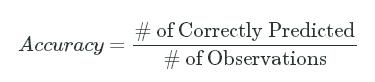
Prediction accuracy boils down to the number of labels that were correctly predicted divided by the total number of observations:

Accuracy=# of Correctly Predicted# of ObservationsAccuracy=# of Correctly Predicted# of Observations

Instructions

• Train a logistic regression model using the gpa column from thetrain Dataframe.
• Use the LogisticRegression method predict to return the predicted labels for the gpacolumn from the testDataframe. Assign the resultinglist of labels to thepredicted_label column in thetest Dataframe.
• Calculate the accuracy of the predictions by dividing the number of rows whereactual_label matchespredicted_label by the total number of rows in the test set.
• Assign the accuracy value toaccuracy and display it using theprint function.

shuffled_index = np.random.permutation(admissions.index)
shuffled_admissions = admissions.loc[shuffled_index]
train = shuffled_admissions.iloc[0:515]
test = shuffled_admissions.iloc[515:len(shuffled_admissions)]
from sklearn.linear_model import LogisticRegression
model=LogisticRegression()
model.fit(train[["gpa"]],train["actual_label"])
labels=model.predict(test[["gpa"]])
test["predicted_label"]=labels
matches=test["predicted_label"]==test["actual_label"]
correct_predictions=test[matches]
accuracy=len(correct_predictions)/len(test)
print(accuracy)

 

4: Sensitivity And Specificity

Looks like the prediction accuracy is about 63.6%, which isn't too far off from the accuracy value we computed in the previous mission of64.6%. If the model performed significantly worse on new data, this means that it's overfitting. If the prediction accuracy was much lower, say 40% instead of 69%, we would reconsider using logistic regression.

When we evaluated the model on the training data in the previous mission, we achieved a sensitivity value of 12.7% and a specificity value of 96.3%. Let's calculate these measures for the test set and compare. Here's a quick refresher of sensitivity and specificity:

• Sensitivity helps us answer the question:
  • How effective is this model at identifying positive outcomes?
  • Of all of the students that should have been admitted (True Positives + False Negatives), how many did the model correctly admit (True Positives)?
• Specificity helps us answer the question:
  • How effective is this model at identifying negative outcomes?
  • Of all of the applicants who should have been rejected (False Positives + True Negatives), what proportion were correctly rejected (just True Negatives).

Now it's your turn! Calculate the specificity and sensitivity values for the predictions on the test set. To encourage you to avoid relying on the formulas for these measures, we've hidden the exact formula in the Hint and prefer that you work backwards from the goals of these measures instead.

Instructions

• Calculate the sensitivity value for the predictions on the test set and assign to sensitivity.
• Calculate the specificity value for the predictions on the test set and assign to specificity.
• Display both values using theprint function.

 

model = LogisticRegression()
model.fit(train[["gpa"]], train["actual_label"])
labels = model.predict(test[["gpa"]])
test["predicted_label"] = labels
matches = test["predicted_label"] == test["actual_label"]
correct_predictions = test[matches]
accuracy = len(correct_predictions) / len(test)
true_positives=len(test[(test["actual_label"]==1)&(test["predicted_label"]==1)])
False_negatives=len(test[(test["actual_label"]==1)&(test["predicted_label"]==0)])
sensitivity=true_positives/(true_positives+False_negatives)
true_negative=len(test[(test["actual_label"]==0)&(test["predicted_label"]==0)])
false_positives=len(test[(test["actual_label"]==0)&(test["predicted_label"]==1)])
specificity=true_negative/(false_positives+true_negative)
print(specificity)
print(sensitivity)

 

5: False Positive Rate

It turns out that our test set achieved a sensitivity value of 8.3, compared to a sensitivity value of 12.7% from the previous mission, and a specificity value of 96.3%, which matches the specificity value of 96.3% from the previous mission. We have a little more evidence now that our logistic regression model is able to generalize to new data.

So far, we've been using the LogisticRegression method predict to generate predictions for labels. For each observation, scikit-learn uses the logit function, with the optimal parameter value for the data the model was trained on, to return a probabillity value. If the probability value is larger than 50%, the predicted label is 1 and if it's less than 50%, the predictd label is 0. For most problems, however, 50% is not the optimal discrimination threshold. We need a way to vary the threshold and compute the measures at each threshold. Then, depending on the measure we want to optimize, we can find the appropriate threshold to use for predictions.

The 2 common measures that are computed for each discrimination threshold are the False Positive Rate (or fall-out) and the True Positive Rate (or sensitivity). While we've explored the latter measure, we haven't discussed fall-out:

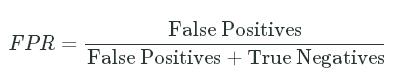
• Fall-out or False Positive Rate - The proportion of applicants who should have been rejected (actual_label equals 0) but were instead admitted (predicted_label equals 1):

FPR=False PositivesFalse Positives+True NegativesFPR=False PositivesFalse Positives+True Negatives

These 2 rates describe how well the model accepts the right students and how poorly it rejects the wrong one:

• True Positive Rate: The proportion of students that were admitted that should have been admitted.
• False Positive Rate: The proportion of students that were accepted that should have been rejected.

import matplotlib.pyplot as plt
%matplotlib inline

from sklearn import metrics
probabilities=model.predict_proba(test[["gpa"]])
fpr, tpr, thresholds = metrics.roc_curve(test["actual_label"], probabilities[:,1])
plt.plot(fpr,tpr)

6: ROC Curve

We can vary the discrimination threshold and calculate the TPR and FPR for each value. This is called an ROC curve, which stands for reciever operator curve, and it allows us to understand a classification model's performance as the discrimination threshold is varied. To calculate the TPR and FPR values at each discrimination threshold, we can use the scikit-learn roc_curve function. This function will calculate the false positive rate and true positive rate for varying discrimination thresholds until both reach 0%.

This function takes 2 required parameters:

• y_true: list of the true labels for the observations,
• y_score: list of the model's probability scores for those observations.

As the example code in the documentation suggests, the roc_curve function returns 3 values which you can assign all at once:

fpr, tpr, thresholds = metrics.roc_curve(labels, probabilities)

You'll notice that the returned thresholds won't usually range from 0.0 to 1.0 and will instead constrains the result set to the minimum range where FPR and TPR range from 0.0 to 1.0. Once we have the FPR and TPR for each relevant threshold, we can plot the ROC curve using the Matplotlib plot function.

Instructions

• Import the relevant scikit-learn package you need to calculate the ROC curve.
• Use the model to return predicted probabilities for the test set.
• Use the roc_curve function to return the FPR and TPR values for different thresholds.
• Create and display a line plot with:
  • the FPR values on the x-axis and
  • the TPR values on the y-axis.

# Note the different import style!
from sklearn.metrics import roc_auc_score

probabilities=model.predict_proba(test[["gpa"]])
auc_score=roc_auc_score(test["actual_label"],probabilities[:,1])
print(auc_score)

 

8: Next Steps

With an AUC score of about 57.8%, our model does a little bit better than 50%, which would correspond to randomly guessing, but not as high as the university may like. This could imply that using just one feature in our model, GPA, to predict admissions isn't enough. All of the measures and scores we've learned about are different ways of thinking about accuracy and the important takeaway is that no single measure will tell us if we want to use a specific model or not. Understanding how individual scores are calculated and what they focus on help you converge onto a clearer picture. It's always important to understand what measures are the most important for the problem at hand.

In the next mission, we'll switch gears and learn how we can use machine learning on problems that don't involve predicting a label. This type of machine learning is called unsupervised machine learning and we'll focus on a technique called clustering.