一、显式微分方程

clc,clear
tspan = [0:10];
y0 = 2;
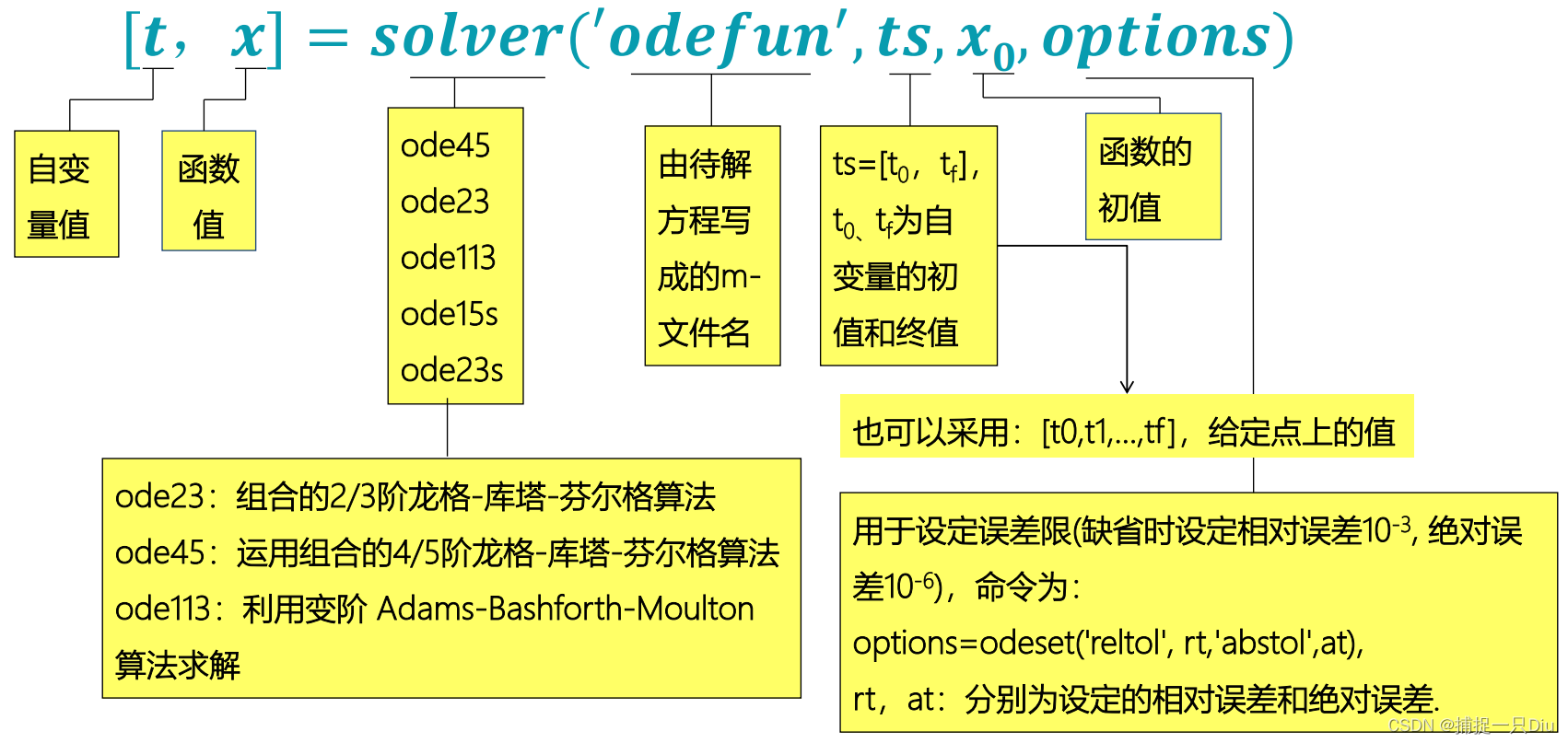
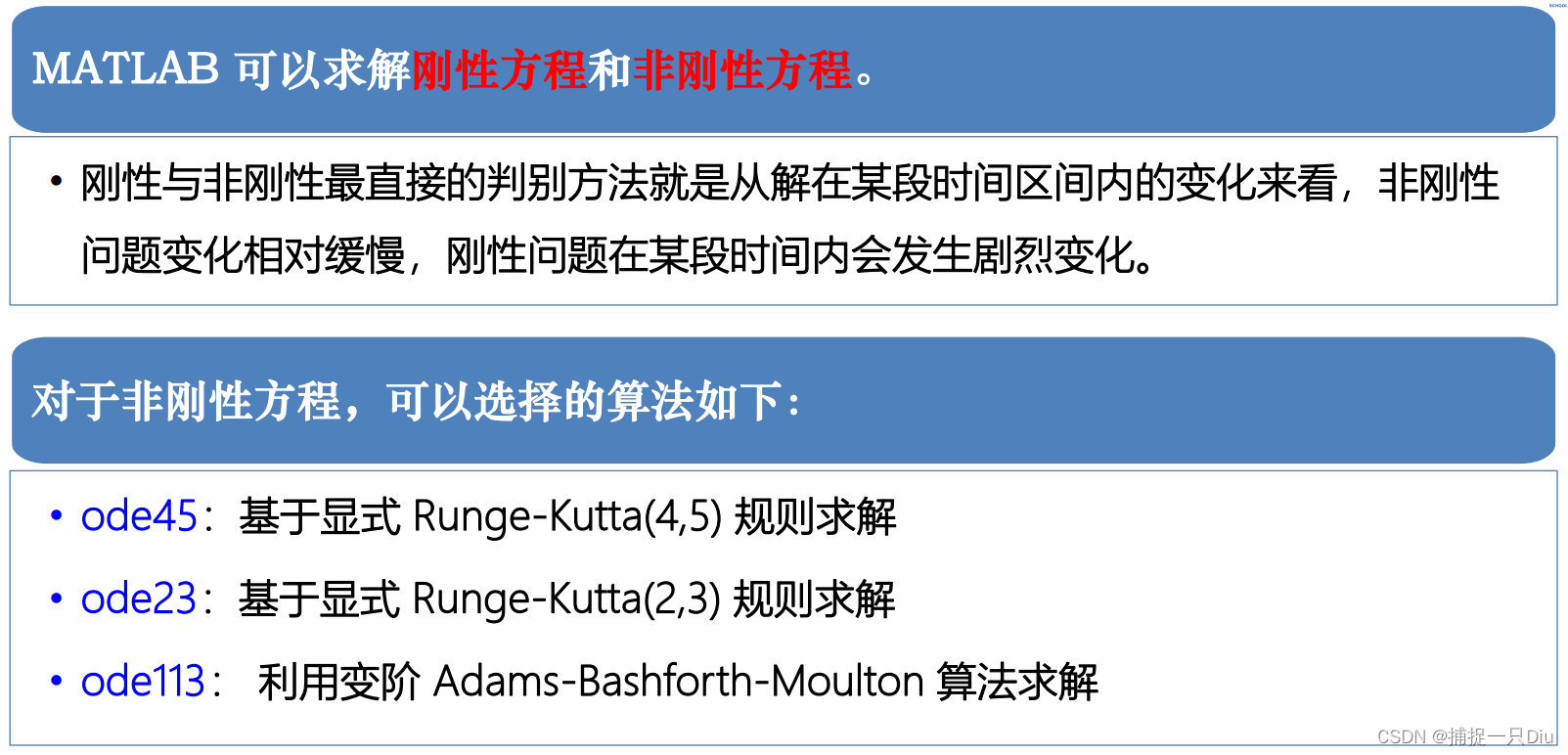
[t1,y1] = ode23(@odefun_1,tspan,y0); %求数值解,精度相对低
[t2,y2] = ode113(@odefun_1,tspan,y0); %求数值解,精度相对高
yt = sqrt(tspan'+1)+1; %求精确解
subplot(1,2,1)
plot(t1,y1,'bo',t2,y2,'r*',tspan,yt,'g-')
legend('ode23求解','ode113求解','精确解','Location','best');
subplot(1,2,2)
y1t = abs(y1-yt);
y2t = abs(y2-yt);
plot(t1,y1t,'bo',t2,y2t,'r*')
legend('ode23误差','ode113误差','Location','best');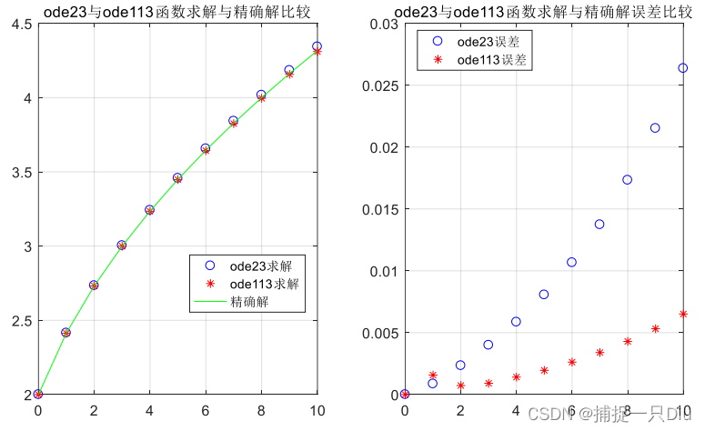
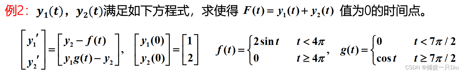
function dydt = odefun_2(t,y)
    ft = 2*sin(t).*(t<4*pi) + 0.*(t>=4*pi); %定义分段函数f(t)
    gt = cos(t).*(t>=3.5*pi) + 0.*(t<3.5*pi); %定义分段函数g(t)
    dydt = [y(2) - ft;
           y(1)*gt-y(2)]; %微分方程组
end
ts = [0,20];
y0 = [1,2];
sol = ode23tb(@odefun_2,ts,y0)
subplot(1,2,1)
plot(sol.x,sol.y(1,:),'b-','LineWidth',1.5)
hold on
plot(sol.x,sol.y(2,:),'r--','LineWidth',1.5)
grid on
legend('{\ity}_1(t)','{\ity}_2(t)','Location','best')
legend('boxoff')
title('微分方程组解的曲线')
xlabel('t')
ylabel('y')
ysum = sum(sol.y);
subplot(1,2,2)
plot(sol.x,ysum,'b-','LineWidth',1.5)
hold on
fplot(@(t)0*t,[0,20])
fh = @(t)sum(deval(sol,t));
[x01,y01] = fzero(fh,10)
[x02,y02] = fzero(fh,18)
plot(x01,y01,'r.','MarkerSize',15)
hold on
plot(x02,y02,'r.','MarkerSize',15)
grid on
legend('F(t) = {\ity}_1(t) + {\ity}_2(t)','y = 0的直线','Location','best');
legend('boxoff')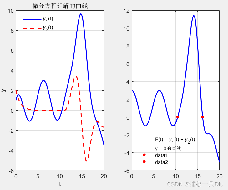

function dy = DyDtFun(t,y)
    dy = zeros(3,1);
    dy(1) = y(2)*y(3);
    dy(2) = -y(1)*y(3);
    dy(3) = -0.51*y(1)*y(2);
end
[T,Y]=ode45(@DyDtFun,[0 12],[0 1 1]);
plot(T,Y(:,1),'b:',T,Y(:,2),'g--',T,Y(:,3),'r.-','LineWidth',1.5)
grid on
legend('y_1','y_2','y_3')
legend('boxoff')
title('显示微分方程组初值问题求解')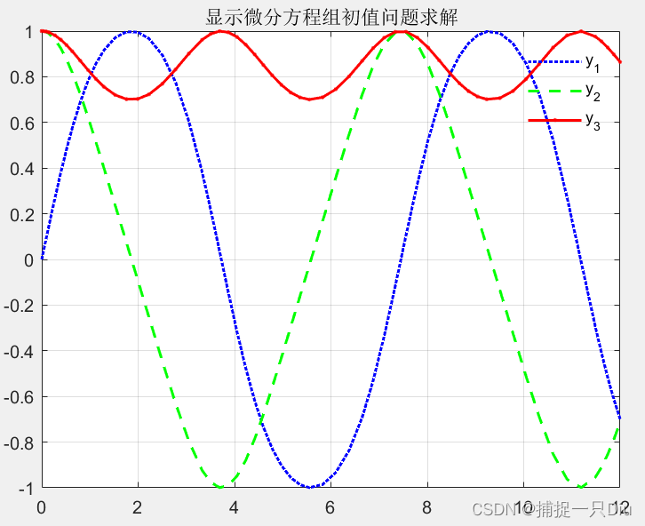
![]()
function dydt = odefun_3(t,y) %定义函数文件
    dydt = [y(2);
           (1-y(1)^2)*y(2)-y(1)];
end
[t,y]=ode45(@odefun_3,[0 20],[2 0]);
plot(t,y(:,1),'b--',t,y(:,2),'r:','LineWidth',1.5);
grid on
title('常微分方程的解');
xlabel('t')
ylabel('y')
legend('y(t)','dy/dt','Location','best')
legend('boxoff')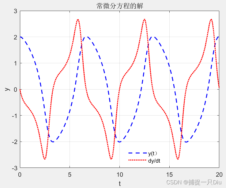
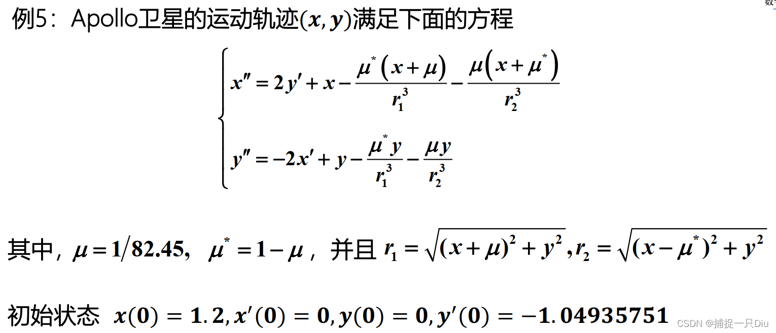
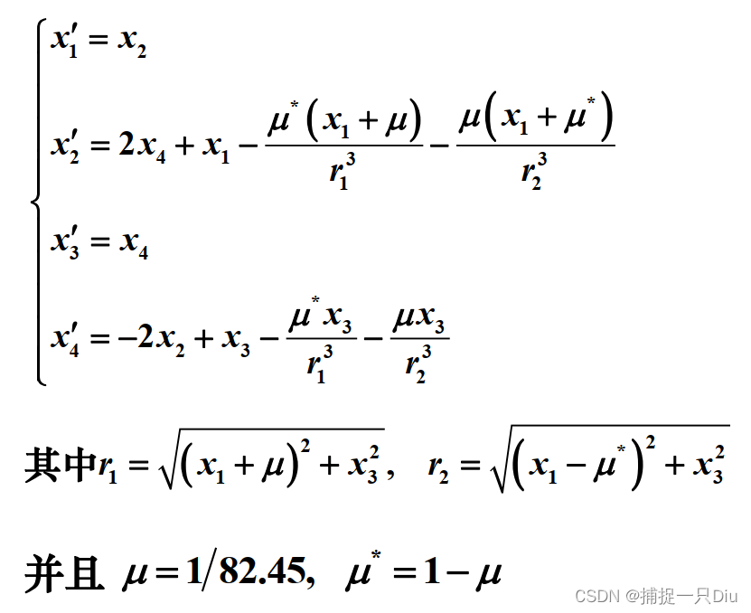
function dxdt = apolloeq(t,x)
    mu = 1/82.45;
    mu1 = 1 - mu;
    r1 = sqrt((x(1)+mu).^2 + x(3).^2);
    r2 = sqrt((x(1)-mu1).^2 + x(3).^2);
    dxdt = [x(2);
            2*x(4) + x(1) - mu1*(x(1) + mu)/r1.^3 - mu*(x(1) - mu1)/r2.^3;
            x(4);
           -2*x(2) + x(3) - mu1*x(3)/r1.^3 - mu*x(3)/r2.^3];
end
x0 = [1.2;0;0;-1.04935751];
% [t,y] = ode45(@apolloeq,[0,20],x0);
[t,y] = ode45(@apolloeq,[0,20],x0,odeset('RelTol',1e-6));
plot(y(:,1), y(:,3),'LineWidth',2)
grid on
title('Apollo卫星的运动轨迹求解图像')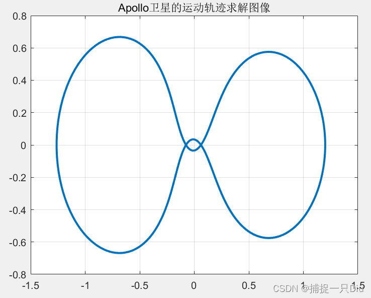
看课后案例分析。
二、完全隐式微分方程

function dydt = odeifun_1(t,y,yp)
    dydt = t.*y.^2.*yp.^3 - y.^3.*yp.^2 + t.*(t.^2 + 1).*yp - t.^2.*y;
end
clc,clear
t0 = 1;
y0 = sqrt(3/2);
ypo = 0;
[y0,yp0] = decic(@odeifun_1,t0,y0,1,ypo,0)
%求得y0 = 1.2247 yp0 = 0.8165
[t,y] = ode15i(@odeifun_1,[1,10],y0,yp0,odeset('RelTol',1e-5));
plot(t,y)
hold on
plot(t,sqrt(t.^2+0.5),'r*') %绘制精确解散点
legend('y=ode15i','y=sqrt(t.^2+0.5)')
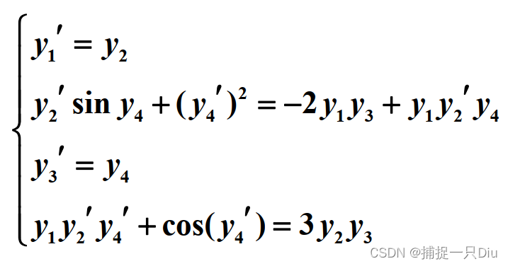
function dydt = odeifun_2(t,y,dy)
dydt = [dy(1)-y(2);
        dy(2)*sin(y(4))+dy(4)^2 + 2*y(1)*y(3)-y(1)*dy(2)*y(4);
        dy(3)-y(4);
        y(1)*dy(2)*dy(4)+cos(dy(4))-3*y(2)*y(3)];
end
t0 = 0;
y0 = [1;0;0;1];
fix_y0 = ones(4,1);
dy0 = [0 3 1 0]';
fix_dy0 = zeros(4,1);
[y02,dy02] = decic(@odeifun_2,t0,y0,fix_y0,dy0,fix_dy0);
[t y] = ode15i(@odeifun_2,[0 5],y02,dy02);
plot(t,y(:,1),'k-',t,y(:,2),'r--', t,y(:,3),'g-.',t,y(:,4),'b:','linewidth',2)
grid on
legend('{\ity}_1(t)','{\ity}_2(t)','{\ity}_3(t)','{\ity}_4(t)','Location','best')
title('隐式微分方程组的解曲线')
xlabel('t')
ylabel('y')
legend('boxoff')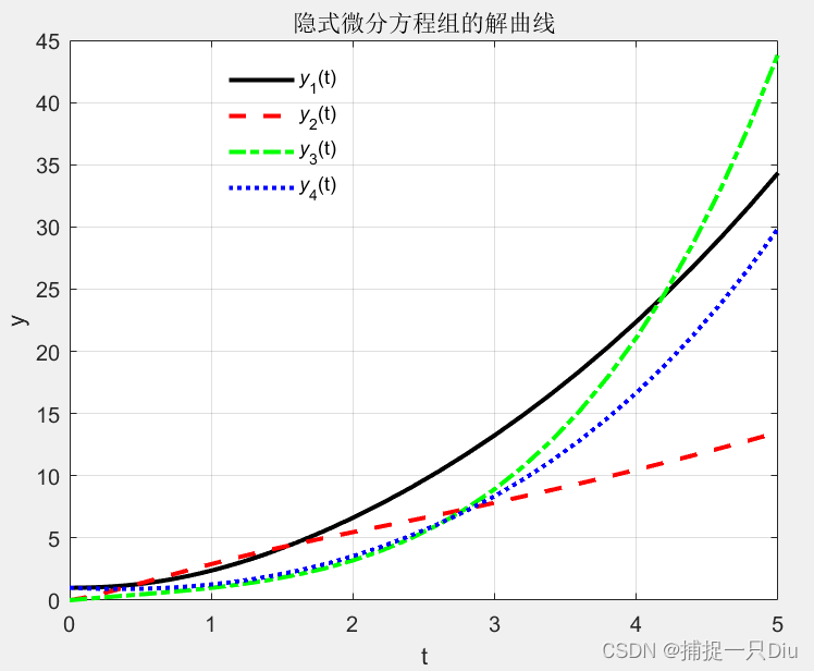
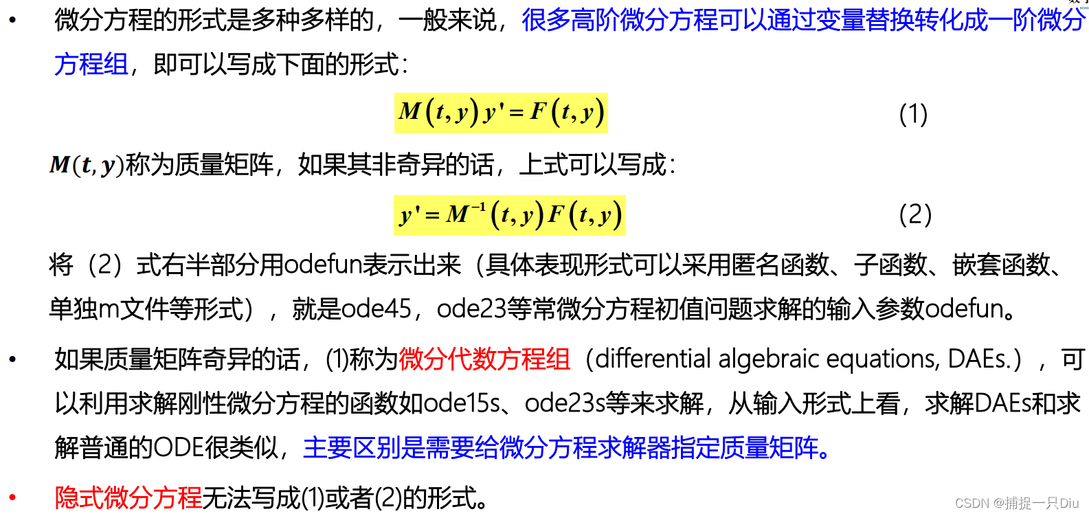
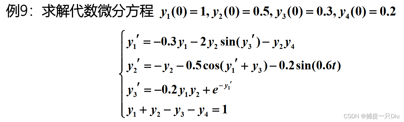
三、代数微分方程组(DAEs)
ode15s用于求显式的微分方程组
![]()
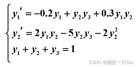
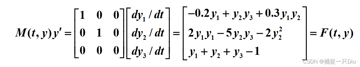
y0 = [0.8;0.1;0.1]; %初值
M = [1 0 0;0 1 0;0 0 0]; %质量矩阵
options = odeset('Mass',M,'RelTol',1e-4,'AbsTol',[1e-6,1e-6,1e-6]);
tspan = [0 20];
[T,Y] = ode15s(@DAEsfun_1,tspan,y0,options);
plot(T,Y(:,1),'b-','linewidth',2)
hold on
plot(T,Y(:,2),'r-.','linewidth',2)
plot(T,Y(:,3),'g:','linewidth',2)
legend('{\ity}_1(t)','{\ity}_2(t)','{\ity}_3(t)','Location','best');
title('代数微分方程求解结果图')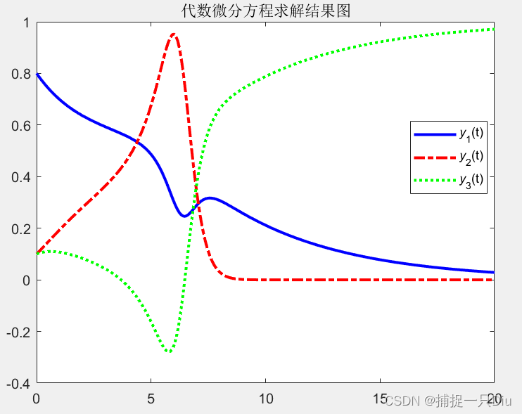
ode15i用于求隐式的微分方程组
function dydt = iDAEsfun_2(t,y,yp)
    % 注意与显式微分方程组定义的不同
    dydt = [yp(1)+0.3*y(1)+2*y(2).*sin(yp(3))+y(2).*y(4);
            yp(2)+y(2)+0.5*cos(yp(1)+y(3))+0.2*sin(0.6*t);
            yp(3)+0.2*y(1).*y(2)-exp(-yp(1));
            y(1)+y(2)-y(3)-y(4)-1];
end
y0 = [1;0.5;0.3;0.2]; % 初值
tspan = [0 5]; % 求值区间
fix_y0 = [0;1;1;1];
fix_yp0 = [0;0;0;0]; % 该组初值都可以改变,故全部为0
% fsolve
fh = @(y)[y(1)+0.4+sin(y(3)),y(2)+0.5+0.5*cos(y(1)+0.3),y(3)+0.1-exp(y(1))];
fsolve(fh,[1,1,1]) % -0.7596 -0.9481 0.3678
yp0 = [-0.8;-1;1;1];
% 首先求yp0,使得f(t,y,yp) = 0
[y02,yp02] = decic(@iDAEsfun_2,0,y0,fix_y0,yp0,fix_yp0)
[t,y] = ode15i(@iDAEsfun_2,tspan,y02,yp02);
plot(t,y(:,1),'k-',t,y(:,2),'r-.',t,y(:,3),'b:',t,y(:,4),'g--','linewidth',1.5)
grid on
legend('{\ity}_1(t)','{\ity}_2(t)','{\ity}_3(t)','{\ity}_4(t)','Location','best')
legend('boxoff')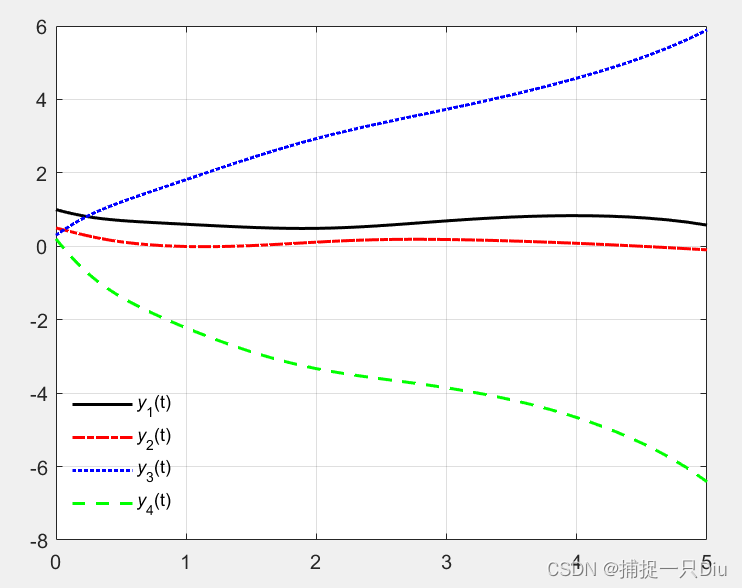
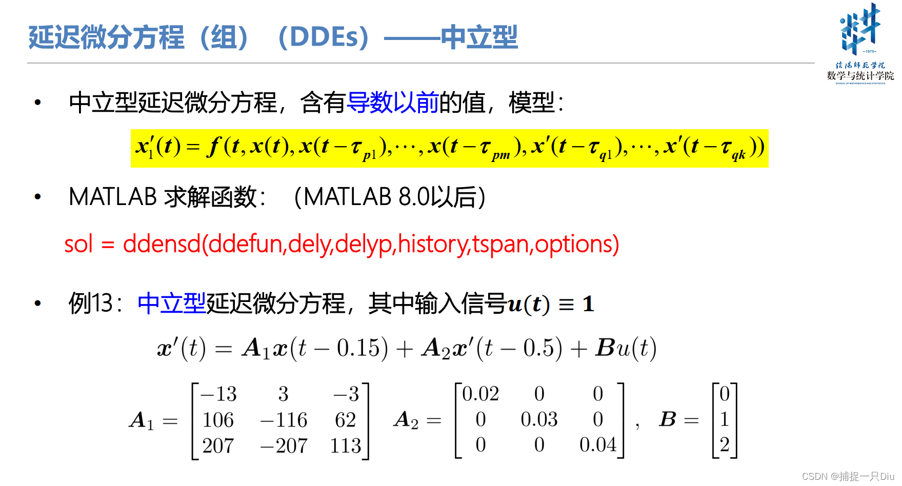
四、延时/时滞微分方程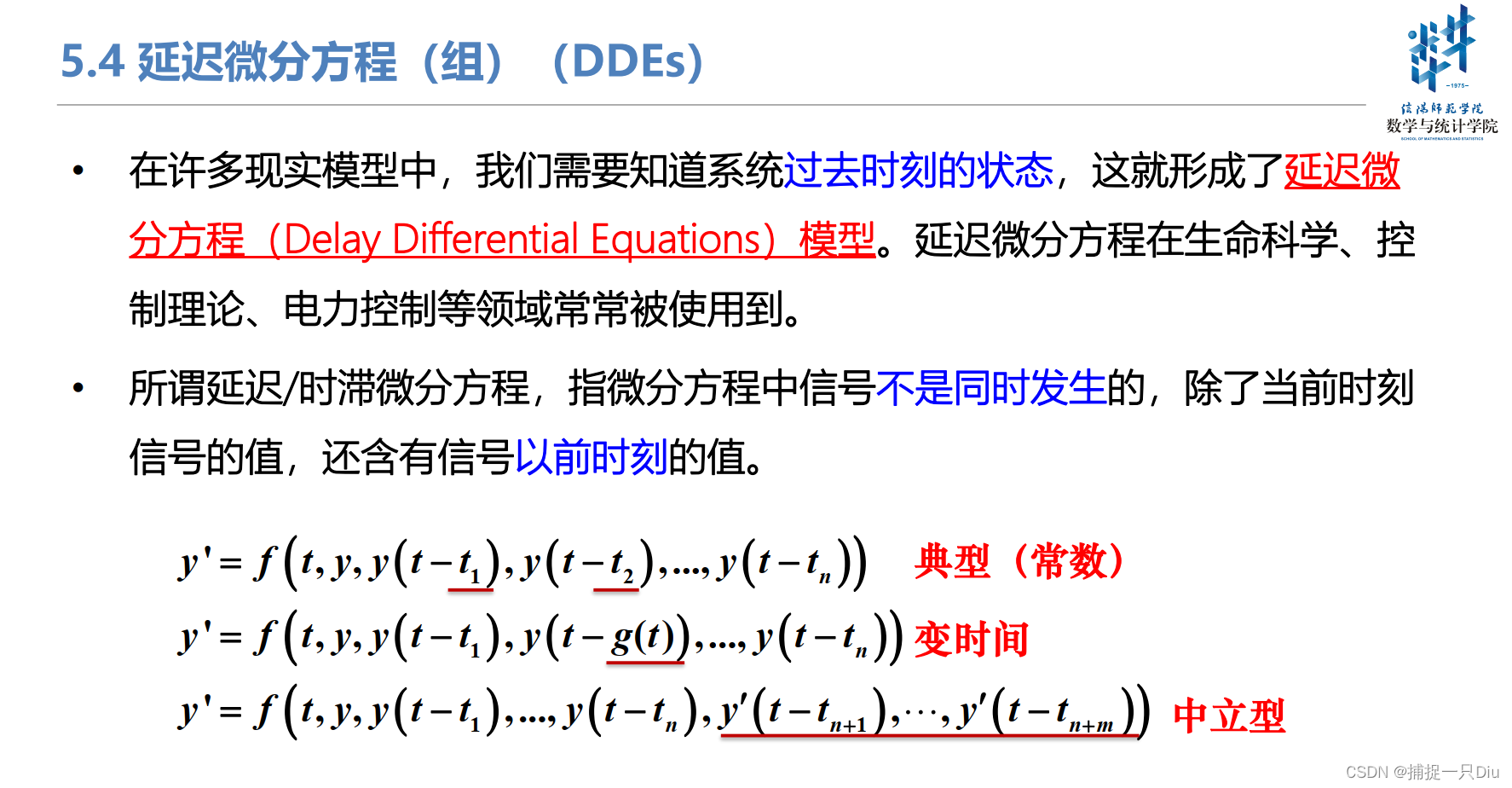
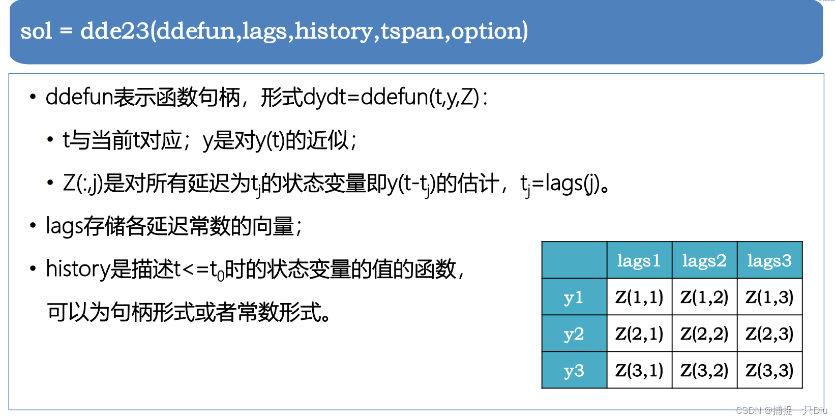

显式微分方程
function dydt = DDEsfun_1(t,y,Z)
    dydt = [0.5*Z(3,2) + 0.5*y(2).*cos(t);
            0.3*Z(1,1) + 0.7*y(3).*sin(t);
            y(2) + cos(2*t)];
end
lags = [1,3]; % 延迟常数向量
history = [0,0,1]; % 小于初值时的历史函数
tspan = [0,8];
sol = dde23(@DDEsfun_1,lags,history,tspan) % 调用dde23求解
ti = 0:0.01:8;
% yi = deval(sol,ti);
% plot(ti,yi(1,:),ti,yi(2,:),ti,yi(3,:))
plot(sol.x,sol.y(1,:),'r-','linewidth',2);
hold on
grid on
plot(sol.x,sol.y(2,:),'b-.','linewidth',2)
plot(sol.x,sol.y(3,:),'g-*','linewidth',1)
legend('{\ity}_1(t)','{\ity}_2(t)','{\ity}_3(t)','Location','best')
title('方程各解的曲线图')
legend('boxoff')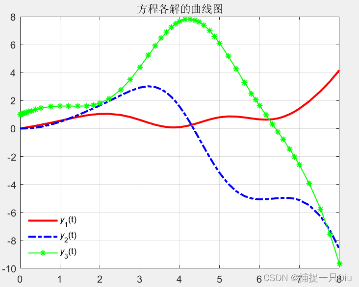

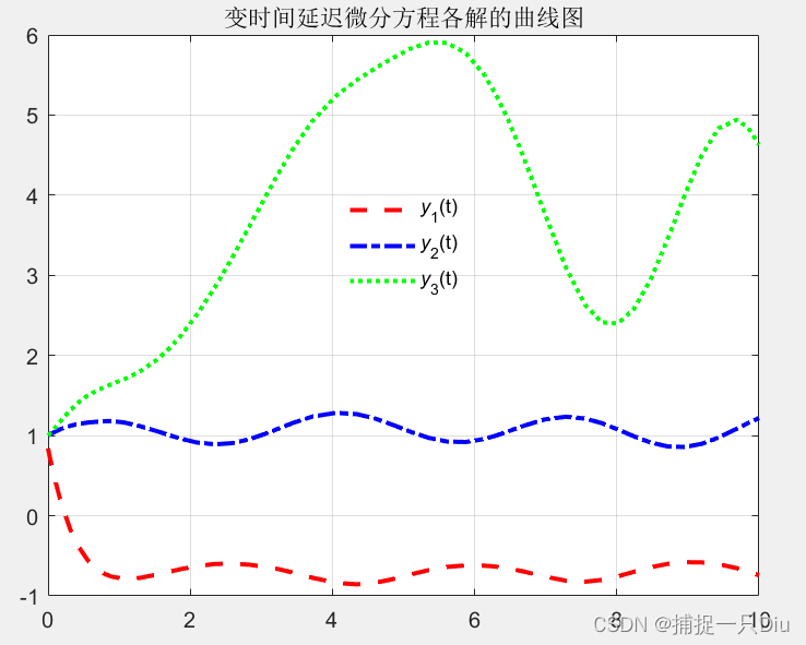
function dydt = DDEsfun_2(t,x,Z)
    dydt = [-2*x(2) - 3*Z(1,1);
            -0.05*x(1).*x(3) - 2*Z(2,2) + 2;
            0.3*x(1).*x(2).*x(3) + cos(x(1).*x(2)) + 2*sin(0.1*t.^2)];
end
lags = @(t,x)[t - 0.2*abs(sin(t)); t - 0.8];
history = zeros(3,1);
tspan = [0,10];
sol = ddesd(@DDEsfun_2,lags,history,tspan)
plot(sol.x,sol.y(1,:),'r--',sol.x,sol.y(2,:),'b-.',sol.x,sol.y(3,:),'g:','linewidth',2);
legend('{\ity}_1(t)','{\ity}_2(t)','{\ity}_3(t)','Location','best')
legend('boxoff')
grid on
title('变时间延迟微分方程各解的曲线图')

lags = @(t,x)[t - 0.2*abs(sin(t)); t - 0.8];
% history = zeros(3,1);
history = @(t,x)[sin(t+1); cos(t); exp(3*t)];
tspan = [0,10];
sol = ddesd(@DDEsfun_2,lags,history,tspan)
% ti = 0:0.01:10;
% yi = deval(sol,ti);
% plot(ti,yi(1,:),'r--',ti,yi(2,:),'b-.',ti,yi(3,:),'g:','linewidth',2)
plot(sol.x,sol.y(1,:),'r--',sol.x,sol.y(2,:),'b-.',sol.x,sol.y(3,:),'g:','linewidth',2)
legend('{\ity}_1(t)','{\ity}_2(t)','{\ity}_3(t)','Location','best')
legend('boxoff')
grid on
title('变时间延迟微分方程各解的曲线图')
function dxdt = DDEsfun_3(t,x,Z,ZP)
    A1 = [-13 3 -3; 106 -116 62; 207 -207 113];
    A2 = diag([0.02 0.03 0.04]);
    B = [0;1;2];
    U = 1;
    dxdt = A1*Z + A2*ZP + B*U;
end
history = zeros(3,1);
sol = ddensd(@DDEsfun_3,0.15,0.5,history,[0,15])
plot(sol.x,sol.y(1,:),'r--',sol.x,sol.y(2,:),'b-.',sol.x,sol.y(3,:),'g:','linewidth',2)
legend('{\ity}_1(t)','{\ity}_2(t)','{\ity}_3(t)','Location','best')
legend('boxoff')
grid on
title('中立型延迟微分方程组解曲线')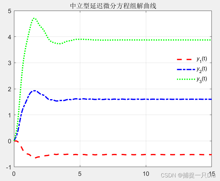
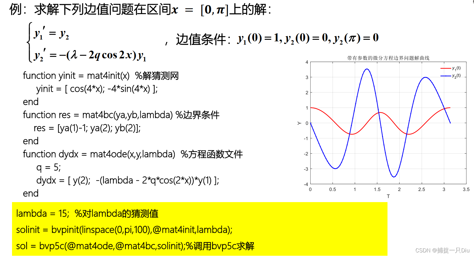
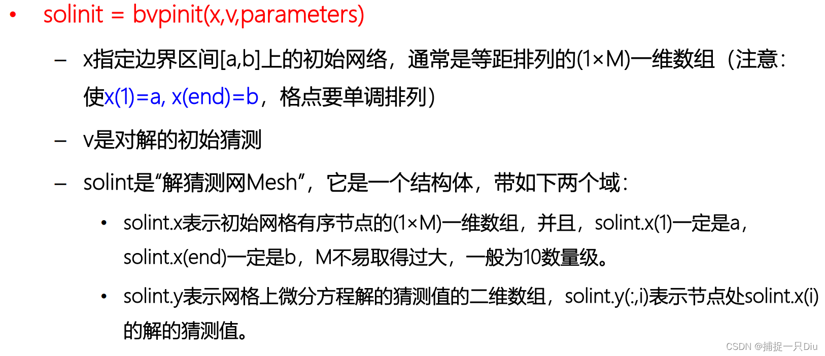
五、微分方程边值问题
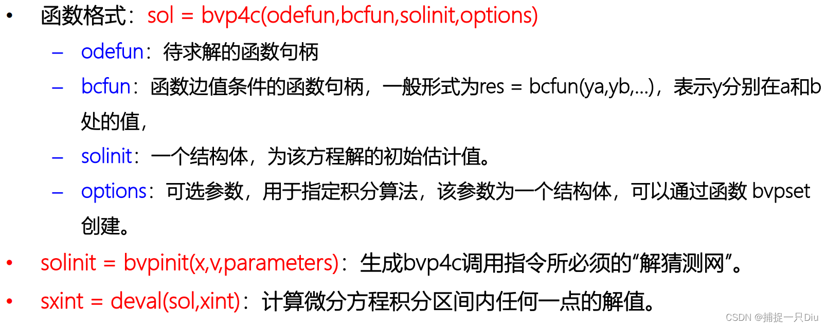
solinit: solve initial.

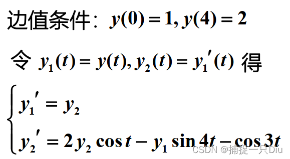
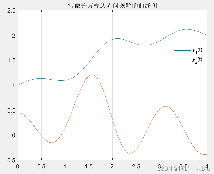
function dydt = bvpfun_1(t,y)
    dydt = [y(2);
            2*y(2).*cos(t) - y(1).*sin(4*t) - cos(3*t)];
end
function res = bcfun_1(ya,yb)
res = [ya(1) - 1;
yb(1) - 2];
endfunction yint = initfun_1(t)
% y(0) = 1, y(4) = 2 --> (0,1),(4,2)
yint = [1/4*t + 1;
1/4]
endfunction dfdy = jacb(t,y)
dfdy = [0, 1;
-sin(4*t), 2*cos(t)];
endsolinit = bvpinit(linspace(0,4,10),@initfun_1)
opts = bvpset('FJacobian',@jacb,'RelTol',1e-4,'AbsTol',1e-8,'Stats','on');
sol = bvp4c(@bvpfun_1,@bcfun_1,solinit,opts)
sol5 = bvp5c(@bvpfun_1,@bcfun_1,solinit,opts)
% bvp5c精度比bvp4c高
ti = 0:0.01:4;
yi = deval(sol,ti);
plot(ti,yi(1,:),ti,yi(2,:))
grid on
legend('{\ity}_1(t)','{\ity}_2(t)','Location','best')
legend('boxoff')
title('常微分方程边界问题解的曲线图')