目录
一、数据介绍
二、下载数据
三、可视化数据
四、模型构建
五、模型训练
六、模型预测
一、数据介绍
MNIST数据集是深度学习入门的经典案例,因为它具有以下优点:
1. 数据量小,计算速度快。MNIST数据集包含60000个训练样本和10000个测试样本,每张图像的大小为28x28像素,这样的数据量非常适合在GPU上进行并行计算。
2. 标签简单,易于理解。MNIST数据集的标签只有0-9这10个数字,相比其他图像分类数据集如CIFAR-10等更加简单易懂。
3. 数据集已标准化。MNIST数据集中的图像已经被归一化到0-1之间,这使得模型可以更快地收敛并提高准确率。
4. 适合初学者练习。MNIST数据集是深度学习入门的最佳选择之一,因为它既不需要复杂的数据预处理,也不需要大量的计算资源,可以帮助初学者快速上手深度学习。
综上所述,MNIST数据集是深度学习入门的经典案例,它具有数据量小、计算速度快、标签简单、数据集已标准化、适合初学者练习等优点,因此被广泛应用于深度学习的教学和实践中。
手写数字识别技术的应用非常广泛,例如在金融、保险、医疗、教育等领域中,都有很多应用场景。手写数字识别技术可以帮助人们更方便地进行数字化处理,提高工作效率和准确性。此外,手写数字识别技术还可以用于机器人控制、智能家居等方面 。
使用torch.datasets.MNIST下载到指定目录下:./data,当download=True时,如果已经下载了不会再重复下载,同train选择下载训练数据还是测试数据
官方提供的类:
class MNIST(
    root: str,
    train: bool = True,
    transform: ((...) -> Any) | None = None,
    target_transform: ((...) -> Any) | None = None,
    download: bool = False
)
Args:
    root (string): Root directory of dataset where MNIST/raw/train-images-idx3-ubyte
        and MNIST/raw/t10k-images-idx3-ubyte exist.
    train (bool, optional): If True, creates dataset from train-images-idx3-ubyte,
        otherwise from t10k-images-idx3-ubyte.
    download (bool, optional): If True, downloads the dataset from the internet and
        puts it in root directory. If dataset is already downloaded, it is not downloaded again.
    transform (callable, optional): A function/transform that takes in an PIL image
        and returns a transformed version. E.g, transforms.RandomCrop
    target_transform (callable, optional): A function/transform that takes in the
        target and transforms it.
二、下载数据
# 导入数据集
# 训练集
import torch
from torchvision import datasets,transforms
from torch.utils.data import Dataset
train_loader = torch.utils.data.DataLoader(
    datasets.MNIST(root="./data",
                   train=True,
                   download=True,
                   transform=transforms.Compose([transforms.ToTensor(),transforms.Normalize((0.1307,),(0.3081,))])),
                    batch_size=64,
                    shuffle=True)

# 测试集
test_loader = torch.utils.data.DataLoader(
    datasets.MNIST("./data",train=False,transform=transforms.Compose([transforms.ToTensor(),transforms.Normalize((0.1307,),(0.3081,))])),
    batch_size=64,shuffle=True
)
pytorch也提供了自定义数据的方法,根据自己数据进行处理
使用PyTorch提供的Dataset和DataLoader类来定制自己的数据集。如果想个性化自己的数据集或者数据传递方式,也可以自己重写子类。
以下是一个简单的例子,展示如何创建一个自定义的数据集并将其传递给模型进行训练:
import torch
from torch.utils.data import Dataset, DataLoader

class MyDataset(Dataset):
    def __init__(self, data, labels):
        self.data = data
        self.labels = labels

    def __len__(self):
        return len(self.data)

    def __getitem__(self, index):
        x = self.data[index]
        y = self.labels[index]
        return x, y

data = torch.randn(100, 3, 32, 32)
labels = torch.randint(0, 10, (100,))

my_dataset = MyDataset(data, labels)
my_dataloader = DataLoader(my_dataset, batch_size=4, shuffle=True)
详细完整流程可参考: Pytorch快速搭建并训练CNN模型?
三、可视化数据
mport matplotlib.pyplot as plt
import numpy as np
import torchvision
def imshow(img):
    img = img / 2 + 0.5 # 逆归一化
    npimg = img.numpy()
    plt.imshow(np.transpose(npimg,(1,2,0)))
    plt.title("Label")
    plt.show()

# 得到batch中的数据
dataiter = iter(train_loader)
images,labels = next(dataiter)
# 展示图片
imshow(torchvision.utils.make_grid(images))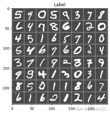
四、模型构建
定义模型类并继承nn.Module基类
# 构建模型
import torch.nn as nn
import torch
import torch.nn.functional as F
class MyNet(nn.Module):
    def __init__(self):
        super(MyNet,self).__init__()
        # 输入图像为单通道,输出为六通道,卷积核大小为5×5
        self.conv1 = nn.Conv2d(1,6,5)
        self.conv2 = nn.Conv2d(6,16,5)
        # 将16×4×4的Tensor转换为一个120维的Tensor,因为后面需要通过全连接层
        self.fc1 = nn.Linear(16*4*4,120)
        self.fc2 = nn.Linear(120,84)
        self.fc3 = nn.Linear(84,10)

    def forward(self,x):
        # 在(2,2)的窗口上进行池化
        x = F.max_pool2d(F.relu(self.conv1(x)),2)
        x = F.max_pool2d(F.relu(self.conv2(x)),2)
        # 将维度转换成以batch为第一维,剩余维数相乘为第二维
        x = x.view(-1,self.num_flat_features(x))
        x = F.relu(self.fc1(x))
        x = F.relu(self.fc2(x))
        x = self.fc3(x)
        return x

    def num_flat_features(self,x):
        size = x.size()[1:]
        num_features = 1
        for s in size:
            num_features *= s
        return num_features

net = MyNet()
print(net)
输出:
MyNet(
  (conv1): Conv2d(1, 6, kernel_size=(5, 5), stride=(1, 1))
  (conv2): Conv2d(6, 16, kernel_size=(5, 5), stride=(1, 1))
  (fc1): Linear(in_features=256, out_features=120, bias=True)
  (fc2): Linear(in_features=120, out_features=84, bias=True)
  (fc3): Linear(in_features=84, out_features=10, bias=True)
)
简单的前向传播
# 前向传播
print(len(images))
image = images[:2]
label = labels[:2]
print(image.shape)
print(image.size())
print(label)
out = net(image)
print(out)
输出:
16
torch.Size([2, 1, 28, 28])
torch.Size([2, 1, 28, 28])
tensor([6, 0])
tensor([[ 1.5441e+00, -1.2524e+00,  5.7165e-01, -3.6299e+00,  3.4144e+00,
          2.7756e+00,  1.1974e+01, -6.6951e+00, -1.2850e+00, -3.5383e+00],
        [ 6.7947e+00, -7.1824e+00,  8.8787e-01, -5.2218e-01, -4.1045e+00,
          4.6080e-01, -1.9258e+00,  1.8958e-01, -7.7214e-01, -6.3265e-03]],
       grad_fn=<AddmmBackward0>)
计算损失:
# 计算损失
# 因为是多分类,所有采用CrossEntropyLoss函数,二分类用BCELoss
image = images[:2]
label = labels[:2]
out = net(image)
criterion = nn.CrossEntropyLoss()
loss = criterion(out,label)
print(loss)
输出:
tensor(2.2938, grad_fn=<NllLossBackward0>)五、模型训练
# 开始训练
model = MyNet()
# device = torch.device("cuda:0")
# model = model.to(device)
import torch.optim as optim
optimizer = optim.SGD(model.parameters(),lr=0.01) # lr表示学习率
criterion = nn.CrossEntropyLoss()
def train(epoch):
    # 设置为训练模式:某些层的行为会发生变化(dropout和batchnorm:会根据当前批次的数据计算均值和方差,加速模型的泛化能力)
    model.train()
    running_loss = 0.0
    for i,data in enumerate(train_loader):
        # 得到输入和标签
        inputs,labels = data
        # 消除梯度
        optimizer.zero_grad()
        # 前向传播、计算损失、反向传播、更新参数
        outputs = model(inputs)
        loss = criterion(outputs,labels)
        loss.backward()
        optimizer.step()
        # 打印日志
        running_loss += loss.item()
        if i % 100 == 0:
            print("[%d,%5d] loss: %.3f"%(epoch+1,i+1,running_loss/100))
            running_loss = 0

train(10)
输出:
[11,    1] loss: 0.023
[11,  101] loss: 2.302
[11,  201] loss: 2.294
[11,  301] loss: 2.278
[11,  401] loss: 2.231
[11,  501] loss: 1.931
[11,  601] loss: 0.947
[11,  701] loss: 0.601
[11,  801] loss: 0.466
[11,  901] loss: 0.399
六、模型预测
# 模型预测结果
correct = 0
total = 0
with torch.no_grad():
    for data in test_loader:
        images,labels = data
        outputs = model(images)
        # 最大的数值及最大值对应的索引
        value,predicted = torch.max(outputs.data,1)
        total += labels.size(0)
        # 对bool型的张量进行求和操作,得到所有预测正确的样本数,采用item将整数类型的张量转换为python中的整型对象
        correct += (predicted == labels).sum().item()
    print("predicted:{}".format(predicted[:10].tolist()))
    print("label:{}".format(labels[:10].tolist()))
    print("Accuracy of the network on the 10 test images: %d %%"% (100*correct/total))

imshow(torchvision.utils.make_grid(images[:10],nrow=len(images[:10])))
输出:
predicted:[1, 0, 7, 6, 5, 2, 4, 3, 2, 6]
label:[1, 0, 7, 6, 5, 2, 4, 8, 2, 6]
Accuracy of the network on the 10 test images: 91 %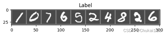
对应类别的准确率:
class_correct = list(0. for i in range(10))
class_total = list(0. for i in range(10))
classes = [i for i in range(10)]

with torch.no_grad():# model.eval()
    for data in test_loader:
        images,labels = data
        outputs = model(images)
        value,predicted = torch.max(outputs,1)
        c = (predicted == labels).squeeze()
        # 对所有labels逐个进行判断
        for i in range(len(labels)):
            label = labels[i]
            class_correct[label] += c[i].item()
            class_total[label] += 1
    print("class_correct:{}".format(class_correct))
    print("class_total:{}".format(class_total))

# 每个类别的指标
for i in range(10):
    print('Accuracy of -> class %d : %2d %%'%(classes[i],100*class_correct[i]/class_total[i]))
输出:
class_correct:[958.0, 1119.0, 948.0, 938.0, 901.0, 682.0, 913.0, 918.0, 748.0, 902.0]
class_total:[980.0, 1135.0, 1032.0, 1010.0, 982.0, 892.0, 958.0, 1028.0, 974.0, 1009.0]
Accuracy of -> class 0 : 97 %
Accuracy of -> class 1 : 98 %
Accuracy of -> class 2 : 91 %
Accuracy of -> class 3 : 92 %
Accuracy of -> class 4 : 91 %
Accuracy of -> class 5 : 76 %
Accuracy of -> class 6 : 95 %
Accuracy of -> class 7 : 89 %
Accuracy of -> class 8 : 76 %
Accuracy of -> class 9 : 89 %