基于WIN10的64位系统演示

一、写在前面

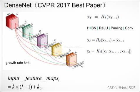
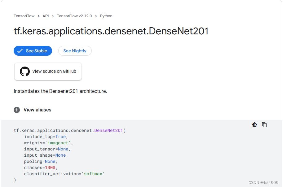
（1）DenseNet201

DenseNet201是一种深度卷积神经网络，是DenseNet网络的一种变体。DenseNet，全称Dense Convolutional Network（密集卷积网络），是由Facebook AI Research在2016年提出的一种卷积神经网络架构。

DenseNet的主要特点是其密集连接的特性。在DenseNet中，每个层都与之前所有层直接连接，每一层的输入不仅包括前一层的输出，而且还包括所有之前层的输出。这种结构可以增强特征的传播，使得网络可以利用所有层的特征信息，有助于改善梯度流和稀疏性学习。

DenseNet201是DenseNet系列中的一种，其结构比DenseNet121更深，拥有201层。这种深度使得DenseNet201在处理图像分类任务时，能够获得更好的性能。其主要优势在于其能够有效地利用特征，减少参数数量，降低过拟合的风险，提高模型的泛化能力。同时，由于其复杂的网络结构，DenseNet201的训练需要较大的计算资源。

（2）DenseNet201的预训练版本

Keras有DenseNet201的预训练模型，省事：

 

二、DenseNet201迁移学习代码实战

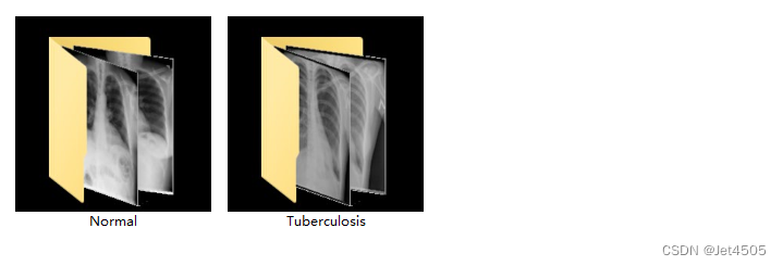
我们换个数据集：肺结核病人和健康人的胸片的识别。其中，肺结核病人700张，健康人900张，分别存入单独的文件夹中。

 

（a）导入包

from tensorflow import keras
import tensorflow as tf
from tensorflow.python.keras.layers import Dense, Flatten, Conv2D, MaxPool2D, Dropout, Activation, Reshape, Softmax, GlobalAveragePooling2D, BatchNormalization
from tensorflow.python.keras.layers.convolutional import Convolution2D, MaxPooling2D
from tensorflow.python.keras import Sequential, initializers
from tensorflow.python.keras import Model
from tensorflow.python.keras.optimizers import adam_v2
import numpy as np
import matplotlib.pyplot as plt
from tensorflow.python.keras.preprocessing.image import ImageDataGenerator, image_dataset_from_directory
from tensorflow.python.keras.layers.preprocessing.image_preprocessing import RandomFlip, RandomRotation, RandomContrast, RandomZoom, RandomTranslation
import os,PIL,pathlib
import warnings
#设置GPU
gpus = tf.config.list_physical_devices("GPU")

if gpus:
    gpu0 = gpus[0] #如果有多个GPU，仅使用第0个GPU
    tf.config.experimental.set_memory_growth(gpu0, True) #设置GPU显存用量按需使用
    tf.config.set_visible_devices([gpu0],"GPU")
    
warnings.filterwarnings("ignore")             #忽略警告信息
plt.rcParams['font.sans-serif'] = ['SimHei']  # 用来正常显示中文标签
plt.rcParams['axes.unicode_minus'] = False    # 用来正常显示负号

（b）导入数据集

#1.导入数据
data_dir = "./MTB"
data_dir = pathlib.Path(data_dir)
image_count = len(list(data_dir.glob('*/*')))
print("图片总数为：",image_count)

batch_size = 32
img_height = 100
img_width  = 100


"""
关于image_dataset_from_directory()的详细介绍可以参考文章：https://mtyjkh.blog.csdn.net/article/details/117018789
"""
train_ds = image_dataset_from_directory(
    data_dir,
    validation_split=0.2,
    subset="training",
    seed=12,
    image_size=(img_height, img_width),
    batch_size=batch_size)

val_ds = image_dataset_from_directory(
    data_dir,
    validation_split=0.2,
    subset="validation",
    seed=12,
    image_size=(img_height, img_width),
    batch_size=batch_size)

class_names = train_ds.class_names
print(class_names)
print(train_ds)


#2.检查数据
for image_batch, labels_batch in train_ds:
    print(image_batch.shape)
    print(labels_batch.shape)
    break

#3.配置数据
AUTOTUNE = tf.data.AUTOTUNE

def train_preprocessing(image,label):
    return (image/255.0,label)

train_ds = (
    train_ds.cache()
    .shuffle(800)
    .map(train_preprocessing)    # 这里可以设置预处理函数
#     .batch(batch_size)           # 在image_dataset_from_directory处已经设置了batch_size
    .prefetch(buffer_size=AUTOTUNE)
)

val_ds = (
    val_ds.cache()
    .map(train_preprocessing)    # 这里可以设置预处理函数
#     .batch(batch_size)         # 在image_dataset_from_directory处已经设置了batch_size
    .prefetch(buffer_size=AUTOTUNE)
)

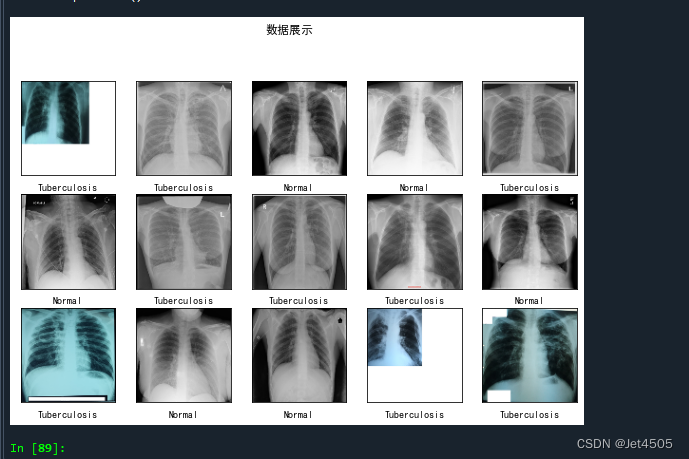
#4. 数据可视化
plt.figure(figsize=(10, 8))  # 图形的宽为10高为5
plt.suptitle("数据展示")

class_names = ["Tuberculosis","Normal"]
for images, labels in train_ds.take(1):
    for i in range(15):
        plt.subplot(4, 5, i + 1)
        plt.xticks([])
        plt.yticks([])
        plt.grid(False)

        # 显示图片
        plt.imshow(images[i])
        # 显示标签
        plt.xlabel(class_names[labels[i]-1])

plt.show()

数据长这样：

 

（c）数据增强

data_augmentation = Sequential([
  RandomFlip("horizontal_and_vertical"),
  RandomRotation(0.2),
  RandomContrast(1.0),
  RandomZoom(0.5,0.2),
  RandomTranslation(0.3,0.5),
])

def prepare(ds):
    ds = ds.map(lambda x, y: (data_augmentation(x, training=True), y), num_parallel_calls=AUTOTUNE)
    return ds
train_ds = prepare(train_ds)

（d）导入DenseNet201

#获取预训练模型对输入的预处理方法
from tensorflow.python.keras.applications.densenet import DenseNet201
from tensorflow.python.keras import Input, regularizers
IMG_SIZE = (img_height, img_width, 3)

base_model = DenseNet201(include_top=False, #是否包含顶层的全连接层
                         weights='imagenet')

inputs = Input(shape=IMG_SIZE)
#模型
x = base_model(inputs, training=False) #参数不变化
#全局池化
x = GlobalAveragePooling2D()(x)
#BatchNormalization
x = BatchNormalization()(x)
#Dropout
x = Dropout(0.8)(x)
#Dense
x = Dense(128, kernel_regularizer=regularizers.l2(0.1))(x)  # 添加 L2 正则化
#BatchNormalization
x = BatchNormalization()(x)
#激活函数
x = Activation('relu')(x)
#输出层
outputs = Dense(2, kernel_regularizer=regularizers.l2(0.1))(x)  # 添加 L2 正则化
#BatchNormalization
outputs = BatchNormalization()(outputs)
#激活函数
outputs = Activation('sigmoid')(outputs)
#整体封装
model = Model(inputs, outputs)
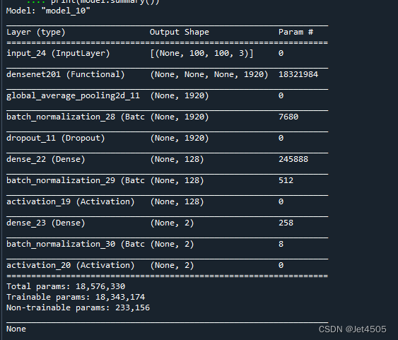
#打印模型结构
print(model.summary())

打印出模型的结构：

 

（e）编译模型

#定义优化器
from tensorflow.python.keras.optimizers import adam_v2, rmsprop_v2
#from tensorflow.python.keras.optimizer_v2.gradient_descent import SGD
optimizer = adam_v2.Adam()
#optimizer = SGD(learning_rate=0.001)
#optimizer = rmsprop_v2.RMSprop()
#编译模型
model.compile(optimizer=optimizer,
                loss='sparse_categorical_crossentropy',
                metrics=['accuracy'])

#训练模型
from tensorflow.python.keras.callbacks import ModelCheckpoint, Callback, EarlyStopping, ReduceLROnPlateau, LearningRateScheduler

NO_EPOCHS = 30
PATIENCE  = 10
VERBOSE   = 1

# 设置动态学习率
annealer = LearningRateScheduler(lambda x: 1e-4 * 0.99 ** (x+NO_EPOCHS))

#性能不提升时，减少学习率
#reduce = ReduceLROnPlateau(monitor='val_accuracy', 
#                           patience=PATIENCE,
#                           verbose=1,
#                           factor=0.8,
#                           min_lr=1e-6)

# 设置早停
earlystopper = EarlyStopping(monitor='loss', patience=PATIENCE, verbose=VERBOSE)

# 
checkpointer = ModelCheckpoint('mtb_jet_best_model_DenseNet201.h5',
                                monitor='val_accuracy',
                                verbose=VERBOSE,
                                save_best_only=True,
                                save_weights_only=True,
                                mode='max')

train_model  = model.fit(train_ds,
                  epochs=NO_EPOCHS,
                  verbose=1,
                  validation_data=val_ds,
                  callbacks=[earlystopper, checkpointer, annealer])

#保存模型
model.save('mtb_jet_best_model_DenseNet201.h5')
print("The trained model has been saved.")

模型训练速度挺快的：

 

（f）Accuracy和Loss可视化

import matplotlib.pyplot as plt

loss = train_model.history['loss']
acc = train_model.history['accuracy']
val_loss = train_model.history['val_loss']
val_acc = train_model.history['val_accuracy']
epoch = range(1, len(loss)+1)

fig, ax = plt.subplots(1, 2, figsize=(10,4))
ax[0].plot(epoch, loss, label='Train loss')
ax[0].plot(epoch, val_loss, label='Validation loss')
ax[0].set_xlabel('Epochs')
ax[0].set_ylabel('Loss')
ax[0].legend()
ax[1].plot(epoch, acc, label='Train acc')
ax[1].plot(epoch, val_acc, label='Validation acc')
ax[1].set_xlabel('Epochs')
ax[1].set_ylabel('Accuracy')
ax[1].legend()
plt.show()

通过这个图，观察模型训练情况：

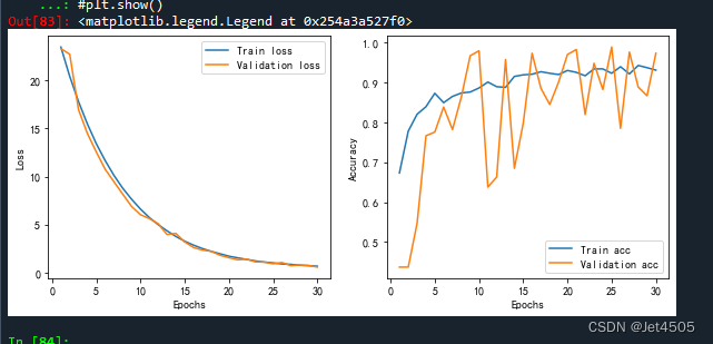
 蓝色为训练集，橙色为验证集。

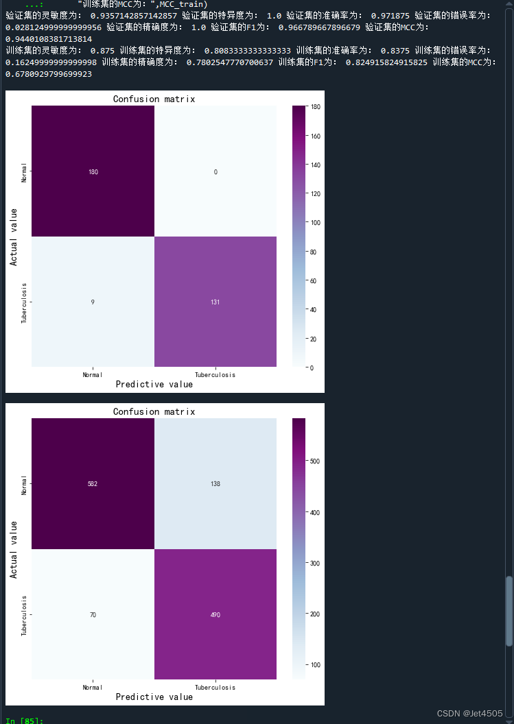
（g）混淆矩阵可视化以及模型参数

没啥好说的，都跟之前的ML模型类似：

import numpy as np
import matplotlib.pyplot as plt
from tensorflow.python.keras.models import load_model
from matplotlib.pyplot import imshow
from sklearn.metrics import classification_report, confusion_matrix
import seaborn as sns
import pandas as pd
import math
# 定义一个绘制混淆矩阵图的函数
def plot_cm(labels, predictions):
    
    # 生成混淆矩阵
    conf_numpy = confusion_matrix(labels, predictions)
    # 将矩阵转化为 DataFrame
    conf_df = pd.DataFrame(conf_numpy, index=class_names ,columns=class_names)  
    
    plt.figure(figsize=(8,7))
    
    sns.heatmap(conf_df, annot=True, fmt="d", cmap="BuPu")
    
    plt.title('混淆矩阵',fontsize=15)
    plt.ylabel('真实值',fontsize=14)
    plt.xlabel('预测值',fontsize=14)

val_pre   = []
val_label = []

for images, labels in val_ds:#这里可以取部分验证数据（.take(1)）生成混淆矩阵
    for image, label in zip(images, labels):
        # 需要给图片增加一个维度
        img_array = tf.expand_dims(image, 0) 
        # 使用模型预测图片中的人物
        prediction = model.predict(img_array)
        val_pre.append(np.argmax(prediction))
        val_label.append(label)

plot_cm(val_label, val_pre)

cm_val = confusion_matrix(val_label, val_pre)    
a_val = cm_val[0,0]
b_val = cm_val[0,1]
c_val = cm_val[1,0]
d_val = cm_val[1,1]
acc_val = (a_val+d_val)/(a_val+b_val+c_val+d_val) #准确率：就是被分对的样本数除以所有的样本数
error_rate_val = 1 - acc_val #错误率：与准确率相反，描述被分类器错分的比例
sen_val = d_val/(d_val+c_val) #灵敏度：表示的是所有正例中被分对的比例，衡量了分类器对正例的识别能力
sep_val = a_val/(a_val+b_val) #特异度：表示的是所有负例中被分对的比例，衡量了分类器对负例的识别能力
precision_val = d_val/(b_val+d_val) #精确度：表示被分为正例的示例中实际为正例的比例
F1_val = (2*precision_val*sen_val)/(precision_val+sen_val) #F1值：P和R指标有时候会出现的矛盾的情况，这样就需要综合考虑他们，最常见的方法就是F-Measure（又称为F-Score）
MCC_val = (d_val*a_val-b_val*c_val) / (math.sqrt((d_val+b_val)*(d_val+c_val)*(a_val+b_val)*(a_val+c_val))) #马修斯相关系数（Matthews correlation coefficient）：当两个类别具有非常不同的大小时，可以使用MCC
print("验证集的灵敏度为：",sen_val, 
      "验证集的特异度为：",sep_val,
      "验证集的准确率为：",acc_val, 
      "验证集的错误率为：",error_rate_val,
      "验证集的精确度为：",precision_val, 
      "验证集的F1为：",F1_val,
      "验证集的MCC为：",MCC_val)
    
train_pre   = []
train_label = []
for images, labels in train_ds:#这里可以取部分验证数据（.take(1)）生成混淆矩阵
    for image, label in zip(images, labels):
        # 需要给图片增加一个维度
        img_array = tf.expand_dims(image, 0)
        # 使用模型预测图片中的人物
        prediction = model.predict(img_array)

        train_pre.append(np.argmax(prediction))
        train_label.append(label)
        
plot_cm(train_label, train_pre)

cm_train = confusion_matrix(train_label, train_pre)  
a_train = cm_train[0,0]
b_train = cm_train[0,1]
c_train = cm_train[1,0]
d_train = cm_train[1,1]
acc_train = (a_train+d_train)/(a_train+b_train+c_train+d_train)
error_rate_train = 1 - acc_train
sen_train = d_train/(d_train+c_train)
sep_train = a_train/(a_train+b_train)
precision_train = d_train/(b_train+d_train)
F1_train = (2*precision_train*sen_train)/(precision_train+sen_train)
MCC_train = (d_train*a_train-b_train*c_train) / (math.sqrt((d_train+b_train)*(d_train+c_train)*(a_train+b_train)*(a_train+c_train))) 
print("训练集的灵敏度为：",sen_train, 
      "训练集的特异度为：",sep_train,
      "训练集的准确率为：",acc_train, 
      "训练集的错误率为：",error_rate_train,
      "训练集的精确度为：",precision_train, 
      "训练集的F1为：",F1_train,
      "训练集的MCC为：",MCC_train)

效果还可以：

 

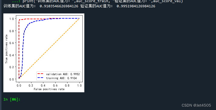
（g）AUC曲线绘制

from sklearn import metrics
import numpy as np
import matplotlib.pyplot as plt
from tensorflow.python.keras.models import load_model
from matplotlib.pyplot import imshow
from sklearn.metrics import classification_report, confusion_matrix
import seaborn as sns
import pandas as pd
import math

def plot_roc(name, labels, predictions, **kwargs):
    fp, tp, _ = metrics.roc_curve(labels, predictions)

    plt.plot(fp, tp, label=name, linewidth=2, **kwargs)
    plt.plot([0, 1], [0, 1], color='orange', linestyle='--')
    plt.xlabel('False positives rate')
    plt.ylabel('True positives rate')
    ax = plt.gca()
    ax.set_aspect('equal')


val_pre_auc   = []
val_label_auc = []

for images, labels in val_ds:
    for image, label in zip(images, labels):      
        img_array = tf.expand_dims(image, 0) 
        prediction_auc = model.predict(img_array)
        val_pre_auc.append((prediction_auc)[:,1])
        val_label_auc.append(label)
auc_score_val = metrics.roc_auc_score(val_label_auc, val_pre_auc)


train_pre_auc   = []
train_label_auc = []

for images, labels in train_ds:
    for image, label in zip(images, labels):
        img_array_train = tf.expand_dims(image, 0) 
        prediction_auc = model.predict(img_array_train)
        train_pre_auc.append((prediction_auc)[:,1])#输出概率而不是标签！
        train_label_auc.append(label)
auc_score_train = metrics.roc_auc_score(train_label_auc, train_pre_auc)

plot_roc('validation AUC: {0:.4f}'.format(auc_score_val), val_label_auc , val_pre_auc , color="red", linestyle='--')
plot_roc('training AUC: {0:.4f}'.format(auc_score_train), train_label_auc, train_pre_auc, color="blue", linestyle='--')
plt.legend(loc='lower right')
#plt.savefig("roc.pdf", dpi=300,format="pdf")

print("训练集的AUC值为：",auc_score_train, "验证集的AUC值为：",auc_score_val)

ROC曲线：

 

三、踩坑过程

开始使用默认的参数跑数据的时候，出现一个问题：

训练集准确率稳步上调，然而验证集准确率稳定在52%不变，且loss为NAN。

咨询了GPT-4，给了一些建议：

（2）数据乱序：代码中在训练数据和验证数据中都使用了.shuffle(1000)，这是正确的做法。然而，在验证数据中进行乱序实际上并不需要，因为在评估模型性能时，数据的顺序并不影响最终结果。这并不是一个错误，只是一种不必要的操作。

我继续追问代码中shuffle的参数如何设置？我的样本为800左右，shuffle取值多少合适？

GPT-4：如果你的样本数只有800，那么理想情况下，你应该将shuffle的参数设置为800，这样可以在每个epoch后，都能完全打乱你的数据集。但这可能会消耗更多的内存。

因此，变动的代码段：

train_ds = (
    train_ds.cache()
    .shuffle(800)
    .map(train_preprocessing)    
    .prefetch(buffer_size=AUTOTUNE)
)
val_ds = (
    val_ds.cache()
.map(train_preprocessing)    
.prefetch(buffer_size=AUTOTUNE)
)

（2）调整学习率：一般情况从0.001开始试逐渐降低，下限为1e-6。

我调整了动态学习率：

# 设置动态学习率
annealer = LearningRateScheduler(lambda x: 1e-4 * 0.99 ** (x+NO_EPOCHS))

这个函数的作用是，随着训练轮数的增加，让学习率以一个指数速率衰减。初始的学习率为0.0001（即1e-4），在每一轮中，学习率都乘以0.99的 (x+NO_EPOCHS) 次方。

（3）调整过拟合：模型存在过拟合，可以尝试调整模型的结构，例如改变全连接层神经元的数量，或者在全连接层之间添加更多的Dropout层。同时，已经使用了L2正则化。

调整如下：

#获取预训练模型对输入的预处理方法
from tensorflow.python.keras.applications.densenet import DenseNet201
from tensorflow.python.keras import Input, regularizers
IMG_SIZE = (img_height, img_width, 3)
base_model = DenseNet201(include_top=False, #是否包含顶层的全连接层
                         weights='imagenet')
inputs = Input(shape=IMG_SIZE)
#模型
x = base_model(inputs, training=False) #参数不变化
#全局池化
x = GlobalAveragePooling2D()(x)
#BatchNormalization
x = BatchNormalization()(x)
#Dropout
x = Dropout(0.8)(x) #参数增加到0.8
#Dense层
x = Dense(128, kernel_regularizer=regularizers.l2(0.1))(x)  # 全连接层减少到128，添加 L2 正则化
#BatchNormalization
x = BatchNormalization()(x)
#激活函数
x = Activation('relu')(x)
#输出层
outputs = Dense(2, kernel_regularizer=regularizers.l2(0.1))(x)  # 添加 L2 正则化
#BatchNormalization
outputs = BatchNormalization()(outputs)
#激活函数
outputs = Activation('sigmoid')(outputs)
#整体封装
model = Model(inputs, outputs)
#打印模型结构
print(model.summary())

体会：经过以上调整，跳出了坑。调参真的是脑力活和体力活，需要进行大量的实验和耐心。而且不同的数据集可能需要不同的策略，需要尝试不同的组合以找到最适合当下数据的方法。

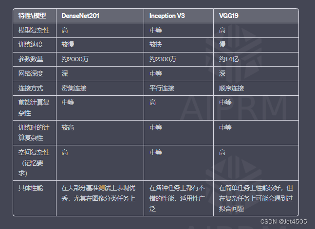
四、DenseNet201和Inception V3、VGG19的对比

 

五、数据

链接：https://pan.baidu.com/s/15vSVhz1rQBtqNkNp2GQyVw?pwd=x3jf

提取码：x3jf